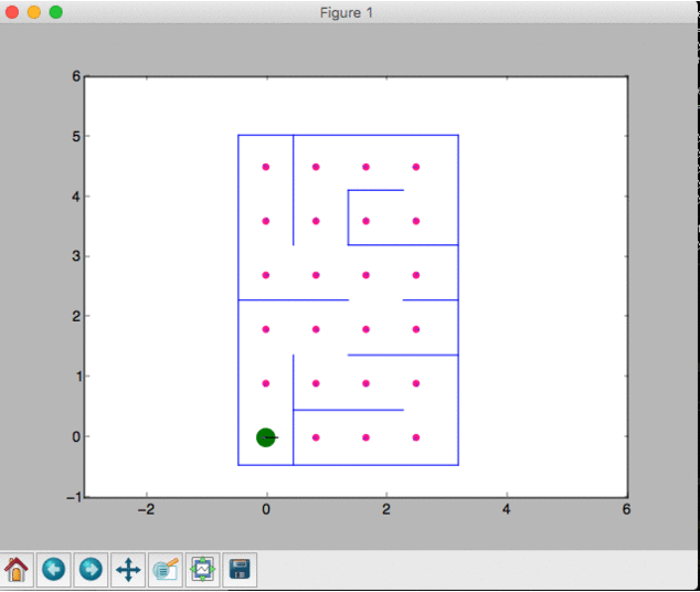
A visualization of how a particle filter can help you locate your robot in a maze… Or just what a particle filter is.

How do we find a lost robot? Well, one method is to use a particle filter to localize the position in a given world.

Background

This was a project that myself, and Tom Wilmots (who is/was also a great basketball player, see here) and Ursula Monaghan (who is also a great field hockey player, see here), worked on for our E28 Mobile Robotics final project. The class was taught by Matt Zucker. You can see some of his work on his blog. Again, if you’re not interested in reading any of this, you can just grab the code here. However, particle filters are a little more complex than like a sudoku solver, so it might be helpful to read some of this!

Matt phrased the final project as such:

In lieu of a final exam, we will have a final project. The final project topic is open-ended, but it must strongly relate to robotics, and it must involve a substantial programming effort.

Each group will give a brief presentation of their project during our scheduled final exam slot on 12/15 from 9AM-12PM.

He also made a few project suggestions, one of which was constructing a particle filter to localize our robot, Leela.

All semester we had been working with TurtleBots, which are essentially glorified Roombas. Totally kidding - Leela was great most of the time. Here’s a video of Leela nudging backwards from a wall. She was still a little jerky then.

Essentially, she’s a humanoid robot.

Theory Behind Particle Filter

Generally

Much of this blog post is going to focus on particle filters with respects to robotics. More generally however, particle filters have many applications and uses. Computationally, it is a form of a genetic algorithm, with particles being scattered around, and then weights being given to said particles, and then sampling in accordance with those weights.

Historically, particle filters belong to the subclass of evolutinary computing, which is a subfield of artificial intelligence. Particle filters even trace back further to the larger field of mean field particle methods. These are a type of Monte Carlo algorithms that are known for satisfying a nonlinear evolution equation. Essentially, this means the updating of the particles is not linear in the sense that often it is random and unpredictable because it depends on the sampling drawn. The big thing to take away here is that there is sequential interacting samples, meaning each of the particles, “interacts with the emperical measures of the process”, as Wikipedia would say.

This type of computing technique is actually, almost unsurprisingly, traced back to Alan Turing in the early 1950’s. Just a fun fact.

Robotics

So in theory, the particle filter is a way to localize your position in a given world, in linear time. This is a big ramp up from a Bayes Filter, which mantains a probability distribution over the entire search space and then updates with a motion and measurement model. This is how we were introduced to it in Mobile Robotics. So then the particle filter is a little bit more clever than the Bayes filter. It’s going to spread particles throughout your maze or map. You can think about these particles as almost baby robots. Then we’re going to get a command, and move all of our particles accordingly, take a measurement around, and give each particle a weight. Then, we resample our particles using those weights as the way to resample. Eventually, if we do a good job with our measurement update and we also do a good job scattering our particles initially, the particles should converge to some degree around the actual position of our robot.

Particle Filter Algorithm

We can really think about this process as occuring in two steps, as Matt laid out in class.

The base starting point is we start with \(n\) particles drawn from some initial distribution. This could be uniform over the entire maze, or some other configuration.

In other words, \(P = \{ x_1, x_2, ... x_{n-1}, x_n \}\) where \(x_i\) is a state in our space.

1. Motion Update

Note, the particle filter samples the motion model. The motion update is relatively simple. We just move each particle from a given command. Let’s call this command \(u\).
So:

\[P' = \{x_1', x_2', ..., x_n' \}\]

where each \(x_i\) is sampled from \(P(x_i ' \mid x_i , u )\).

2. Measurement Update

Note, the particle filter evaluates the measurement model. The measurement update is a little bit more complex. We have to observe our measurement and then we want to know the probability of actually being at such a point. The tricky part is we have to do this for each \(x_i '\) or for each particle. Mathematically speaking, this looks like:

\[w_i = \eta \cdot p(z \mid x_i)\]

where \(\eta\) is the normalizing factor here. So \(\eta = \frac{1}{\sum p(z \mid x_i) }\) . The \(w\)’s are the corresponding weights that result from the measurement model PDF.

But what do these weights mean? They are like little probabilities essentially. So \(w_i\) is the probability that \(x_i '\) is a “good particle”. The good particles are going to align well with the sensor measurements that were reported.

Then! We resample! We assemble \(P = \{ x_1, x_2, ..., x_{n-1}, x_n \}\) by sampling with replacement each \(x_i\) from \(P'\) with probability \(w_i\).

And that’s pretty much it! After this, we just repeat. It’s like a darwinistic approach. So just think about only the best particles from each generation are surviving.

For more information about particle filters, Wikipedia always does a pretty good job.

Raytracer

So in order to get our expected distances, we need to set up a raytracer for our robot. This is how we’re going to get our measurements and evaluate each particle’s position. We can imagine our particle is going look around in the world and we’re going to compare that with the real robot’s perspective as well. If there is a lot of overlap, then the weight is going to be high, because the probability of the robot actually being where the particle is, is also going to be high.

Let’s look at some excerpts of the code.

We have constructed a ray class. It has an origin and direction, both of which are vectors. This is going to be helpful for finding the distance between two rays. That’s the critical problem - in order to find the expected distance, we have our walls (which we constructed as rays), and we have our robot/particle which is shooting out a bunch of rays.

So let’s look at the problem at hand. How do we find the distance between two vectors (and yes, I’m aware that I drew the wall as a line segment, but we wrote the code like a vector)?

For reference, let’s take the above as our diagram.

We can represent the following:

\begin{align} p_i &= p_0 + \alpha \vec{d} \\ p_i &= p_1 + \beta (p_2 - p_1) \end{align}

Let’s rename this vector between \(p_2\) and \(p_1\), as \(\vec{k}\). In other words, \(\vec{k} = p_2 - p_1\)

Then, we can have,

\begin{align} p_i &= p_0 + \alpha \vec{d} \\ p_i &= p_1 + \beta (p_2 - p_1) = p_1 + \beta \vec{k} \end{align}

Then we can relate the two through \(p_i\).

\begin{align} p_1 + \beta \vec{k} &= p_0 + \alpha \vec{d} \\ \alpha \vec{d} - \beta \vec{k} &= p_1 - p_0 \end{align}

Thus relating these in matrix-vector notation.

\[\left[ \begin{array}{c|c} \vec{\mathbf{d}} & -\vec{\mathbf{k}} \end{array} \right] = \left[ \begin{array}{c} \alpha \\ \beta \end{array} \right] = \left[ \begin{array}{c} p_1 \\ -p_0 \end{array} \right]\]

Note, that \(\vec{b}\) and \(\vec{k}\) are actually of shape \(2 \times 1\) as they live in \(\mathbb{R}^2\), therefore the dimensinoality of this will work out. Also note, that we only care about when \(\beta\) lies in the range from [0,1]. If \(\beta\) is not in this range, than we can conclude that there is not a valid intersection. It means that it is not hitting this segment of the wall. We parametrized along our wall with the starting point at \(\beta = 0\) and the ending point at \(\beta = 1\).

With this matrix math set up, we know \(\vec{d}\) and we know \(\vec{k}\). There’s a bunch of different ways that we could solve this problem. We just obviously utilized numpy’s nice built in solver. Specifically, this problem of finding the distance between our robot and the wall segment was really solved by the following short method:

def find_xsection_bn_seg_and_ray(ray, wall_segment):
    p0 = ray.origin
    p1 = wall_segment[0]
    p2 = wall_segment[1]
    
    starting_pt = vec2(p1[0], p1[1])
    ending_pt = vec2(p2[0], p2[1]) 

    k = ending_pt - starting_pt 
    k_vec = np.array([k.getx(), k.gety()])
    d_vec = np.array([ray.direction.getx(), ray.direction.gety()])
    matrix = np.array([d_vec, -k_vec])
    matrix = matrix.transpose()
    
    temp = starting_pt - p0
    p_vec = np.array([temp.getx(), temp.gety()])

    a_b_vec = np.linalg.solve(matrix, p_vec) 

Code

The rest of the code is largely about just iterating over through the particles and calculating the probability and then picking from subsequent probabilities. That’s where the real meat of the particle filter really comes into play. The rest is just making sure that we’re picking the right particle and visualizing everything appropriately.

I will show the measurement and motion update below, but the rest of the code can once again be found here. Feel free to give it a run yourself!

# This is our motion update.
def motion_update(particles, control, sigma_xy, sigma_theta):
    nparticles = particles.shape[1] # how many particles do we have
    noisex = np.random.normal(scale = sigma_xy, size = nparticles) # noise for x
    noisey = np.random.normal(scale = sigma_xy, size = nparticles) # noise for y
    thetanoise = np.random.normal(scale = sigma_theta, size = nparticles) # noise for theta
    if control == "forward":
        particles[0,:] += 3 * FT * np.cos(particles[2,:]) + noisex
        particles[1,:] += 3 * FT * np.sin(particles[2,:]) + noisey
        particles[2,:] += thetanoise
    elif control == "backward":
        particles[0,:] -= 3 * FT * np.cos(particles[2,:]) + noisex
        particles[1,:] -= 3 * FT * np.sin(particles[2,:]) + noisey
        particles[2,:] += thetanoise
    elif control == "turnleft":
        particles[0,:] += noisex
        particles[1,:] += noisey
        particles[2,:] += 90*DEG + thetanoise
    elif control == "turnright":
        particles[0,:] += noisex
        particles[1,:] += noisey
        particles[2,:] -= 90*DEG + thetanoise
    return particles

The above code should make sense with what is being explained in the rest of the article. The motion update is relatively simple. We take a command in - in this case, it is a string of type: forward, backward, turnleft, or turnright. Based on that command, all of the particles are updated accordingly. Note, it is really important that you have a different x and y noise. Otherwise, it could end up looking like this (p.s. sorry about taking screenshots instead of saving the images):

You can see that the noise is now directly correlated. Hence, why the particles now form a linear arrangement across the map. So watch out for your distributions! Besides that, that is all the code you need for the motion update!

# This is our measurement update
def measurement_update(particles, measured_distances):
    # read in our measured distances, just entering this in manually
    z = measured_distances

    # This is so we can alter how many rays we actually want to use
    z = z[::len(z)/NUM_OF_RAYS]
    nan_location = np.isnan(z)

    # our weights should all be the same to start
    weights = np.ones(NUM_OF_PARTICLES)

    # again, get the number of particles... could also use a our global variable
    nparticles = particles.shape[1]

    # ok so here let's iterate over the particles
    for particle_index in range(nparticles):
        expected_distances = help.expected_ranges(particles[:,particle_index], angles_to_use, WALL_SEGS)
        expected_dist = np.array(expected_distances)

        # then we need to iterate over each ray that the particle we're on has seen and compare to the prior 
        for ray_index, val in enumerate(nan_location):
            if val:
                weights[particle_index] = weights[particle_index]
            else:
                weights[particle_index] = weights[particle_index] * \
                    np.exp(-( ( (z[ray_index]-expected_dist[ray_index])**2 ) / (2*SIGMA_Z**2) ) )

    # Need to normalize our weights
    weights = weights / (np.sum(weights))

    # these are the particles that we're going to pick from
    particles_to_use = np.linspace(0, nparticles - 1, num = nparticles)

    # get the indices of the surviving particles
    indices = np.random.choice(particles_to_use, size = nparticles, p = weights)
    indices = indices.astype(int)

    # select the right particles
    particles = particles[:,indices]

    return particles

This is really where the meat of the problem is. Mathematically, computing these weights or probabilities takes the form:

\[w_i = p(z \ | \ x_i ) = \prod_{j=1}^{m} p(z_j \ | \ x_i)\]

So here, the \(x_i\) is the particle’s position in the world. \(m\) is the number of beams that are robot is using. Our z_j is some range for a given ray that is shot out from the robot. In this way, we’re looping over every particle, but then the particle’s probability is the product of all the probabilities for the ray. Hence, why this looks like a double for loop when it’s coded up. One for the particles and one for the rays!

Output

Here’s an output from our program! Note, we displayed the particles after both the motion and measurement update, that’s kind of why the particles jump around a bit.

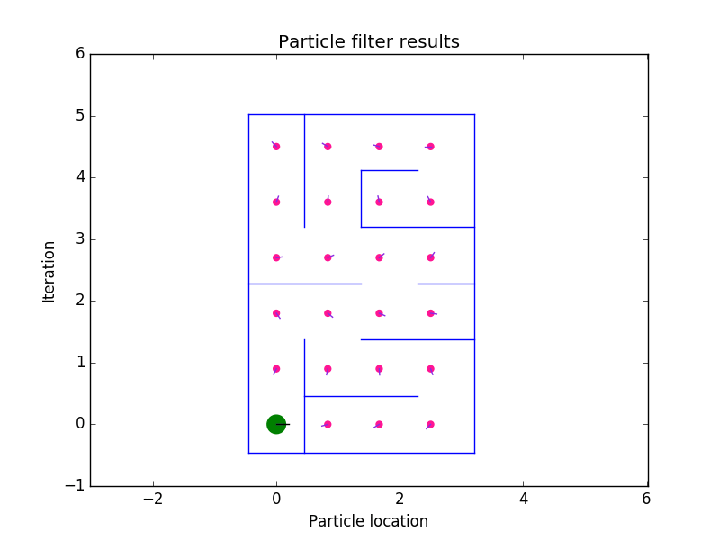
Also ignore the “Iteration” label on the y-axis. I’m just realizing it now, but I don’t want to recreate the gifs again.

Here’s another path!

What’s really really really cool, is that if you watch carefully, when the particles / Leela get to cell (2,1), they kind of hug the bottom most wall. Well, when we were gathering the sensor data from walking Leela through this maze, she actually swung close to that wall. The robot in the visualization doesn’t reflect Leela’s actual position as she traversed (that would have been cool, but hindsight is 20/20). The robot is solely going to the cells that we programmed in. However, the particles are actually adapting to what happened. They swing closer to the wall based on the actual sensor data!! How crazy / cool is that?

Presentation

Finally, we had to present to the class. The presentation pretty much just included everything that this. You can check out our actual presentation, or in the very least a pdf of our presentation here.

Conclusion

Ok so first one big lesson learned:

visual debugging is awesome and will make your life better.

That lesson really got drilled home from Matt after we probably spent an hour trying to debug our code, without realizing that one of the walls we entered was totally incorrect. The other thing that we learned is that genetic algorithms are super interersting. Bayes Theorem has almost limitless applications. Probability is great and I need to learn more. Besides that, it was a really rewarding experience coming up with all of this. As always let me know any comments about my coding style, ways to better my code, corrections to my blog post, etc. Thanks for reading.