This post is going to be focused on discussing how we built our Tennis Scorigami project from a technical standpoint. I’ll discuss the current architecture, some of the design decisions I made, and where I want the project to go next.

If you haven’t yet checked out the main site, feel free to here:

Tennis Scorigami

tennis-scorigami.com

Table of Contents
Motivation
- More Specific Motivation
Demo
Features
Challenges
Surprises
Tech Stack
Engineering + Design
Other Fun Visualizations
- Player Rank History
Conclusion

Motivation

Given once again, the impending collapse of my profession due to automation, my lack of time, and the fact that there’s details on the main website, I will try not to repeat myself.

Our motivation here was largely love of tennis, data, and friendship. Sebastian and Henry were chatting in the groupchat about football scorigami, and Seb asked, I wonder if tennis has any scorigamis. And so, began an interesting conversation, and the groupchat started to explore where we could get data, if anyone had done this and all of that.

More Specific Motivation

More specifically, besides my craving to “wow” my friends, the real pie in the sky goal for us (read: me), was to get Andy Roddick to re-tweet / view this project.

driving-motivation

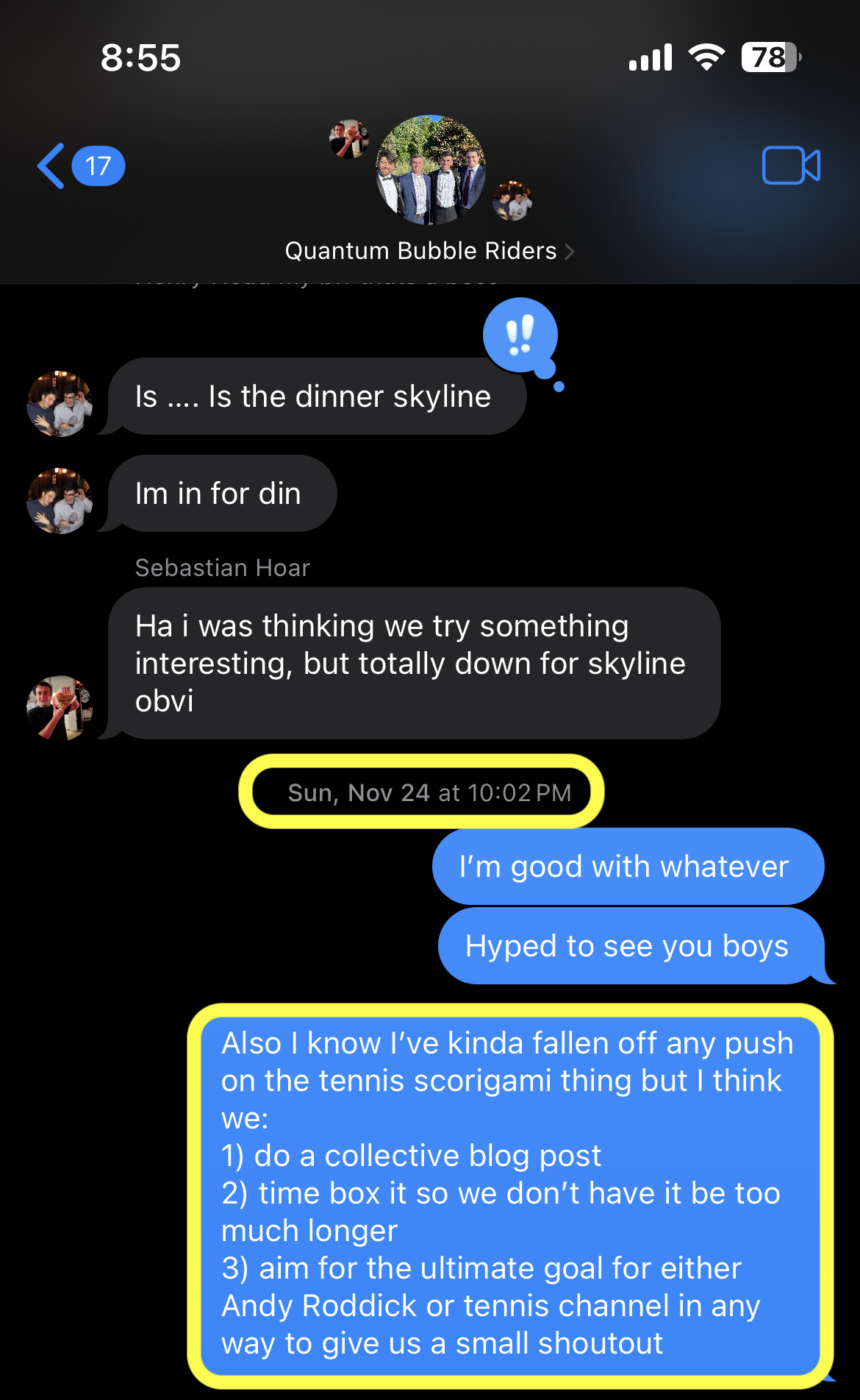
Andy Roddick has been one of our favorite tennis players since growing up, and Henry and I watched as many of his matches as we could get a hold of. So that target was a stretch New Years Resolution of mine.

Demo

If you’re too lazy to visit the website and explore, here’s a demo:

Features

There’s numerous features here that we’re proud of. I’m going to list some of them, and then I’ll discuss them in further detail below:

Graph-Based Score Sequence Modeling
- this was originally Henry’s idea but given how many nodes we have in this search space, it’s not as feasible to just arrange it as a grid like with the NFL
- we thought a graph as a novel (and visually appealing approach)
- what this means technically is that we pre-computed all permutations and did some background processing so that we could store this information in as close to frontend ready format for fast visualization and processing… that gets into our next point
Performance-Optimized Materialized Views
- we built out specific materialized views to help with the performance (given our existing FE filters) so that we can ensure latency is not noticeable
Streaming Visualizations
- Still kind of working on setting this up ideally for 5-graph nodes. There’s 125,062 nodes that we need to render for 5 set match permutations.
- I had to turn to NDJSON (basically just newline json chunked) which I had never used before
- This helped reduce both the latency and the incremental memory on receiving that information and parsing it on the FE
Drizzle
- Ok fair fine you got me. Technically I used both SQLAlchemy and then ported over to Drizzle so that was a little bit of a mess, but I have heard great things about drizzle and liked that experience a lot. drizzle-kit is very sleek and the latest major release for drizzle is fantastic.
(somewhat?) Decent Testing
- Yeah, obviously I wouldn’t say I went crazy here, but I did set up jest, playwright, and storybook
- These are all things that the very talented Michael Barlock first introduced to the team.
- I learned a lot from him and since then, yeah I’ve been trying to incorporate / adopt these a bit more
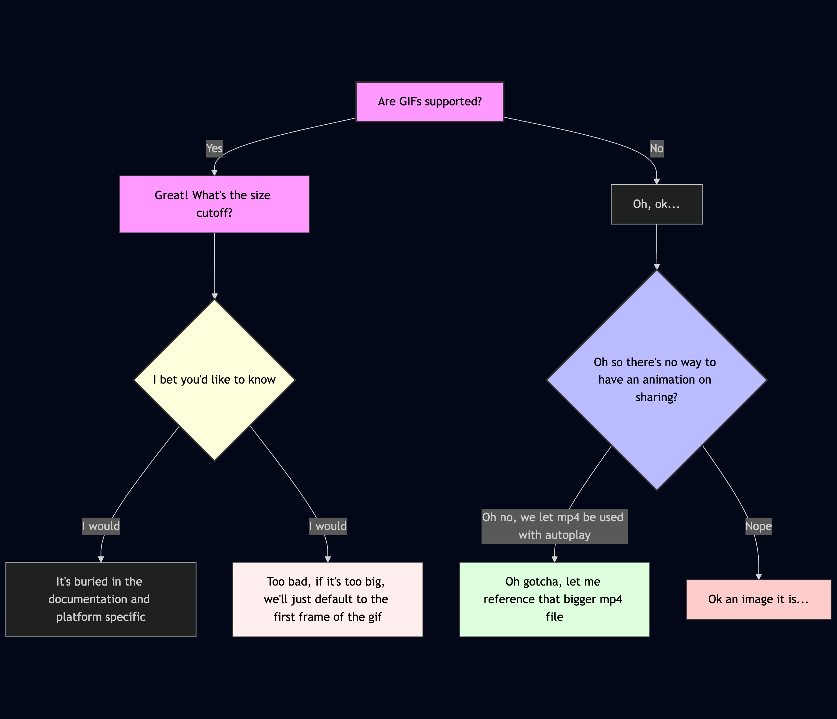
Unfurl Link Coverage
- Perhaps trivial, but try sending https://tennis-scorigami.com/ over iMessage? Yup, it uses the mp4 video with autoplay. What about over Discord? Falls to the native sub-5MB gif that plays. LinkedIn? That same gif? Twitter - just uses a static image as a fallback, and Slack? Also has coverage with the gif / animation support.
- I spent a non-trivial amount on this because it’s the little details that might help Andy Roddick actually click retweet (although yeah I should probably fix that Twitter share link then)

Challenges

Data Consolidation

There's a couple important notes I want to make here.

Our data cutoff is then (partially) hinged on Jeff Sackmann. Currently it's good until the end of 2024. I hate that. I'm not running LLMs, I shouldn't have a data cutoff. I'm planning on building a web scraper for ATP results and setting up my own data feeds because why the f not, and it's 2025 and you can roll (most) software if push really comes to shove. I can go on a full blown rant on my Substack or something, but I am aware of this limitation, and I dislike it more than you.

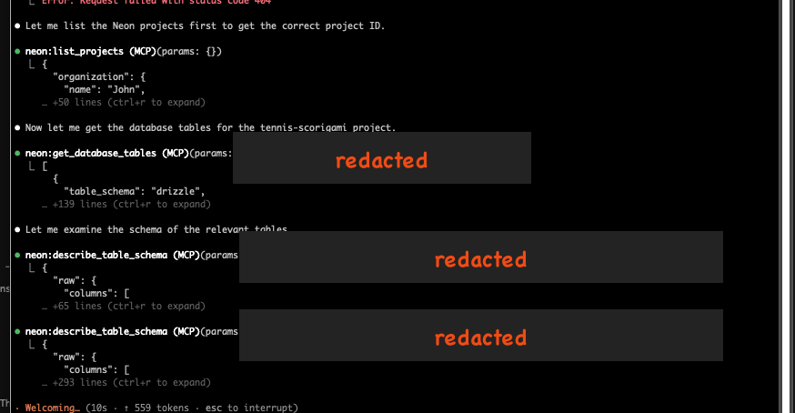
Secondly, consolidating all of this data from disparate sources, always prevents a challenge. There's the age old problem of same logical data, but different source ingestion. I have pulled some of the 2024 matches with SportRadar, and with RapidApi, and with Sackmann, so consolidating that was definitely a bit of elbow grease. Obviously, I used LLMs for parts of this project, but that part was probably the most hands on and driven. Yes, don't worry - I set up my Postgres MCP and after porting to Neon I set up my Neon MCP, but man yeah... still early days I suppose.

Again, as referenced here, tennis data is a commodity. It is insanely annoying and hard to get clean data. I am adamant that another side project that will spin out of this is a publicly available free API for people to query and get tennis data from.

I tried numerous things:

SportRadar
- they’re one of the world’s best data providers
- however, they are absurdly expensive. there’s more info in the Reddit below but they don’t have set plans. as of 2 years ago, for a small time project, they were $1250 a month
- I tried their free trial, ripped as much as I could (of recent tournaments), and then got rate limited, and my trial expired
- Needless to say that was a bit of a miss

API Pricing?
by inSportradar

(continuation)
- one nice thing about SportRadar though was that they publish an OpenAPI (API not AI 🙄) spec of their endpoints.
- You can see their Swagger docs here, and download the openapi.yaml file here
- This made generating a Python client for interacting with it very easy.
- I even created a SportRadar specific Python client for this.
- That repo was (more or less) entirely created with: openapi-python-client generate --path ~/Downloads/openapi.yaml --config tennis-config.yaml with my tennis-config.yaml being as simple as:

project_name_override: sportradar-tennis-v3
package_name_override: sportradar_tennis_v3

Check out the GH repo for the SportRadar client here

Loading repository data...

RapidApi
- Ok but I moved on rapidly (pun intended), because I wasn’t about to pay $1250 a month (unless I was running betting strats)
- I switched to RapidAPI given their generous free plans
- The data quality also suffered here, and a lot of the APIs had pretty stringent API limits (2k calls per month)
- Given this I eventually turned away after pulling what I could
Sackmann
- I seriously need to buy Jeff Sackmann a beer
- He’s consolidated years of tennis data into a decently well organized format
- Sure there’s duplicate players, strange score formats, partial data, conflicts with accents, etc
- Lots of the traditional data quality things, but it’s easier to go from an excess and cleanse than to pull the data out of thin air
- So we stuck with Jeff for our historical data

Being Cheap

This one will be quick, but another challenge of this was just my desire to not spend money. Specifically for a hosted database service. I started with Supabase which I love and use for many other projects, but then pivoted to Aiven which I honestly liked anymore. However, they didn’t have connection pooling and I figured if this did go viral that I would get burned and people would say I was a bad engineer if we were throttling on Aiven’s free plan of like 10 open db transactions. So finally, I ended up Neon because I’ve been wanting to try them and they’re slightly cheaper than Supabase. Here’s an AI generated table summarizing the pros and cons, and decisions:

This table was generated using AI.

Provider	Pros	Cons	Decision Rationale
Supabase	- Great developer experience - Integrated auth + storage - Rich UI/dashboard	- Slightly pricier for scaling - Overhead from extra services if only DB is needed	Preferred for full-stack apps, but overkill + cost when only DB needed
Aiven	- Excellent reliability - Flexible managed Postgres - Simple CLI/tools	- No built-in connection pooling - Free tier limit: ~10 connections	Risky for viral spikes; free tier would throttle app & reflect poorly on eng.
Neon	- Built-in connection pooling - Autoscaling - Cheaper than Supabase - Separation of storage & compute	- Newer platform, less mature - Limited ecosystem/integrations compared to Supabase	Chosen for price/perf tradeoff; avoids pooling issues; good opportunity to test

Fetching 108k Nodes

This was actually pretty fine truth be told in terms of backend performances. The large win of utilizing materialized views was that I could pull the pertinent information, and shape it into the appropriate information that my various FE graph information would require.

Once we get to live data, I’ll set up cronjobs or triggers to refresh these and build out my data pipeline a bit more. However, for the moment, these materialized views were sufficient.

Here’s one as an example:

CREATE MATERIALIZED VIEW public.mv_slug_stats_3_men
TABLESPACE pg_default
AS SELECT s.event_id,
    ss.sequence_id AS id,
    ss.slug,
    ss.depth,
    ss.winner_sets,
    ss.loser_sets,
    is_terminal_3(ss.winner_sets, ss.loser_sets) AS is_terminal,
    3 AS best_of,
    COALESCE(s.played, false) AS played,
    COALESCE(s.occurrences, 0) AS occurrences
   FROM score_sequence ss
     LEFT JOIN mv_sequence_stats_3_men s ON s.sequence_id = ss.sequence_id
  WHERE ss.best_of <= 3
WITH DATA;

-- this is so that we can filter by event_id which is what happens on the frontend when
-- a user selects either a tournament or a year (more or less)
CREATE INDEX idx_mv_slug_stats_3_men_event ON public.mv_slug_stats_3_men USING btree (event_id);

Rendering 108k Nodes

There are numerous repos (some of which I’m using) to help process and render beautiful graphics. I didn’t roll my own physics engine or the force-graph library. I used these:

2D Sigma Graph

Loading repository data...

3D Force Graph

Loading repository data...

Regardless, I wanted a very slick and performant frontend to render all these nodes. The 5 set 3d force graph is not yet built out. You’ll note that vasturiano has a large graph demo here:

And that looks fantastic. However, if you look at the source code…

// https://github.com/vasturiano/react-force-graph/blob/master/example/large-graph/index.html
<head>
  <style> body { margin: 0; } </style>

  <script type="importmap">{ "imports": {
    "react": "https://esm.sh/react",
    "react-dom": "https://esm.sh/react-dom/client"
  }}</script>

<!--  <script type="module">import * as React from 'react'; window.React = React;</script>-->
<!--  <script src="../../src/packages/react-force-graph-3d/dist/react-force-graph-3d.js" defer></script>-->
</head>

<body>
  <div id="graph"></div>

  <script src="//cdn.jsdelivr.net/npm/@babel/standalone"></script>
  <script type="text/jsx" data-type="module">
    import ForceGraph3D from 'https://esm.sh/react-force-graph-3d?external=react';
    import React from 'react';
    import { createRoot } from 'react-dom';

    fetch('../datasets/blocks.json').then(res => res.json()).then(data => {
      createRoot(document.getElementById('graph')).render(
        <ForceGraph3D
          graphData={data}
          nodeLabel={node => <div><b>{node.user}</b>: {node.description}</div>}
          nodeAutoColorBy="user"
          linkDirectionalParticles={1}
        />
      );
    });
  </script>
</body>

And then look at the underlying ../datasets/blocks.json and then do a little bit of Python / json handling… you’ll note:

╭─johnlarkin@Mac ~/Documents/coding/tennis-scorigami ‹feature/john/example-blog-post*›
╰─➤  python                                                                                                                          127 ↵
Python 3.11.7 (v3.11.7:fa7a6f2303, Dec  4 2023, 15:22:56) [Clang 13.0.0 (clang-1300.0.29.30)] on darwin
Type "help", "copyright", "credits" or "license" for more information.
>>> import json
>>> import sys
>>> from pathlib import Path
>>> raw_path = Path('/Users/johnlarkin/Downloads/blocks.json')
>>> raw_content = raw_path.read_text()
>>> data = json.loads(raw_content)
>>> data['nodes'][:2]
[{'id': '4062045', 'user': 'mbostock', 'description': 'Force-Directed Graph'}, {'id': '1341021', 'user': 'mbostock', 'description': 'Parallel Coordinates'}]
>>> len(data['nodes'])
1238 # ... so... not actually that large
>>> len(data['links'])
2602

So… compared to 108k nodes and a similar number of edges… not exactly a port and shift.

However, the 2d sigma graph (with a bit of streaming) can handle this with relative ease. Note, we are playing a bit of a visual game with doing some edge reduction for the farther out layers for 5 graphs, basically following this logic:

edgesToRender = data.edges.filter((edge) => {
  const fromNode = nodeMap.get(edge.frm);
  const toNode = nodeMap.get(edge.to);

  if (!fromNode || !toNode) return false;

  // Always keep early depth edges (structure)
  if (Math.max(fromNode.depth, toNode.depth) <= 2) return true;

  // Keep edges to/from unscored nodes (discovery)
  if (!fromNode.played || !toNode.played) return true;

  // Keep edges with high occurrence nodes
  if (fromNode.occurrences > 100 || toNode.occurrences > 100) return true;

  // For deeper levels, only keep a sample
  return Math.random() < 0.1; // Keep 10% of remaining edges
});

Streaming + NDJSON

However, the crux of keeping the frontend still lightweight for the 5 set rendering was to use NDJSON.

I had heard of NDJSON as a streaming mechanism but hadn’t used it in a production workflow. However, Claude obviously was a huge help here and took care of implementing that part. The crux of the code looks like this:

const response = await fetchGraphStream({
  /* {...filters} */
  maxEdgesPerDepth: GRAPH_CONFIG.maxEdgesPerDepth,
  minOccurrences: GRAPH_CONFIG.minOccurrences,
  signal: abortController.signal,
});

const reader = response.body.getReader();
const decoder = new TextDecoder();
let buffer = "";

/* more code here */

while (true) {
  const { done, value } = await reader.read();
  if (done) break;

  buffer += decoder.decode(value, { stream: true });
  const lines = buffer.split("\n");
  buffer = lines.pop() || "";

  for (const line of lines) {
    if (!line.trim()) continue;

    try {
      const message: StreamMessage = JSON.parse(line);

      switch (message.type) {
        case "meta":
          streamTotalNodes = message.totalNodes;
          streamTotalEdges = message.totalEdges;
          setTotalNodes(streamTotalNodes);
          setTotalEdges(streamTotalEdges);
          /* more code here */
          break;

        case "nodes":
          tempNodes.push(...message.data);
          setLoadedNodes(tempNodes.length);
          /* more code here */
          break;

        case "edges":
          tempEdges.push(...message.data);
          setLoadedEdges(tempEdges.length);
          /* more code here */
          break;

        case "complete":
          setData({ nodes: tempNodes, edges: tempEdges });
          /* more code here */
          break;
      }
    } catch (e) {
      console.error("Failed to parse stream message:", e);
    }
  }
}

How this works is that my backend API route is creating a ReadableStream, basically doing something like this:

const stream = new ReadableStream({...});
return new Response(stream, {...});

Then on the frontend this response.body is that ReadableStream bit, which has the built in getReader() (which returns basically a ReadableStreamDefaultReader).

Then to use that reader, it’s as simple as: const { done, value } = await reader.read();.

This helped a lot for less memory load on the frontend as well as a more interactive and non-blocking call for the UI.

Unfurl Previews

Just a quick note, but the various nuances between different platforms is an absolute headache. Someone needs to sort that out soon. There was basically this decision pipeline for me everytime:

unfurl-decision-tree

Surprises

I was very surprised (and satisfied) when we saw the 8.5 number. 8.5% seemed shockingly low for 5set matches that had been played (tiebreak in the fifth note). So part of it is that 6-0, 0-6 is very uncommon and that opens up a huge part of the search tree to never have been played before. I chatted with ChatGPT or Claude about this as well, and thought its response was interesting (and partially helped me be convinced).

That being said if the was a data quality or data ingestion issue, don't kill the messenger.

There’s numerous reasons for this though. Here are some of them:

there are 108k possible final score outcomes
there have only been 40k 5 set matches in the Open Era
- that’s a rough estimate but I have only loaded in 40k
we’re excluding 2025
- this is exciting, it means there’s lots of scorigamis
concentrated probability distribution
- consider this valid but unlikely scoreline: 6-7, 7-6, 6-0, 1-6, 7-5
- that would require:
  - losing a tiebreak
  - then winning a tiebreak
  - then bageling opponent
  - then getting destroyed 1-6
  - then battle in the final
- this is obviously possible but unlikely at the pro level
order matters
- permutations not combinations! so that increases the space

Here’s an excerpt from the conversation i had with ChatGPT about this:

Below is a concise, self-contained recap of the math followed by a list of reasons the realised coverage is only ≈ 8 %.
The counting
Step What we are counting Result
1. Set-level possibilities A player can win a set by any of seven legal scores (6-0 … 7-6). From the winner’s viewpoint those 7 options are all we need for every set. 7 outcomes per set
2. Match-length patterns Arrange “W” (winner’s set) and “L” (loser’s set) with the last set forced to be W:
• 3-0 → WWW → 1 pattern
• 3-1 → choose where the lone L goes among the first 3 slots ⇒ C(3,1)=3
• 3-2 → choose where the two L’s go among the first 4 slots ⇒ C(4,2)=6 1 + 3 + 6 = 10 patterns
3. Fill each pattern with scores Every set in a k-set pattern has 7 choices ⇒ $7^{k}$.
• 3-set patterns: $7^{3}=343$
• 4-set patterns: $7^{4}=2 401$
• 5-set patterns: $7^{5}=16 807$ multiply per pattern
4. Grand total $\sum \text{patterns}\times 7^{k}$ $1×343 \;+\; 3×2 401 \;+\; 6×16 807 = \boxed{108\,388}$ distinct best-of-5 finals
Why only ~8 % have shown up on court
Matches < boxes The Open-era database has only ≈ 45 000 men’s best-of-5 matches. Even if every one were unique we could fill at most 45 000 / 108 388 ≈ 41 % of the grid. Coverage must start below that ceiling.
Uneven probability mass Tennis scoring is not uniform. Straight-set wins with mundane margins (6-3, 6-4, 6-4) occur constantly, while exotic mixtures such as 6-7, 7-6, 6-0, 1-6, 7-5 require a domination-collapse-rebound sequence that is extraordinarily rare. Most of the 108 388 boxes sit under microscopic probability.
Five-set inflation Five-setters account for 93 % of the theoretical space (16 807 × 6 patterns), yet only about 15 % of real matches go the full distance. That mismatch alone wipes out a huge swath of cells.
Correlation between sets Set scores are not independent draws: if one player is dominating (say 6-1, 6-2) the conditional chance of the next set being a nail-biter (7-6) is lower than the unconditional 1/7. Correlation compresses the practical outcome space far below the naïve $7^{k}$.
Put differently:
\[\text{Observed coverage}\;=\;\frac{\text{≈ 9 200 distinct finals}}{108 388} \;\approx\; 8.5\%.\]
Given the combinatorial overhang, the skewed probability distribution, and the shortfall of five-set matches, landing in the single-digit-percent range is not a surprise—it is the mathematically natural result.

Step	What we are counting	Result
1. Set-level possibilities	A player can win a set by any of seven legal scores (6-0 … 7-6). From the winner’s viewpoint those 7 options are all we need for every set.	7 outcomes per set
2. Match-length patterns	Arrange “W” (winner’s set) and “L” (loser’s set) with the last set forced to be W: • 3-0 → `WWW` → 1 pattern • 3-1 → choose where the lone `L` goes among the first 3 slots ⇒ C(3,1)=3 • 3-2 → choose where the two `L`’s go among the first 4 slots ⇒ C(4,2)=6	1 + 3 + 6 = 10 patterns
3. Fill each pattern with scores	Every set in a k-set pattern has 7 choices ⇒ $7^{k}$. • 3-set patterns: $7^{3}=343$ • 4-set patterns: $7^{4}=2 401$ • 5-set patterns: $7^{5}=16 807$	multiply per pattern
4. Grand total	$\sum \text{patterns}\times 7^{k}$	$1×343 \;+\; 3×2 401 \;+\; 6×16 807 = \boxed{108\,388}$ distinct best-of-5 finals

Tech Stack

Rather than just word vomit what I used here, I’m actually going to just defer to Claude and then summarize with a Mermaid mindmap. What a sentence.

mindmap
  root((Tennis Scorigami))
    Frontend
      Next.js 14
        App Router
        RSC
        API Routes
      React 19
      TypeScript
      Tailwind CSS
        Custom Tennis Theme
        Dark Mode
      UI Libraries
        Radix UI
        Shadcn
      Visualization
        SigmaJS
        3D Force Graph
        Dynamic Imports
      State
        Jotai
        React Query
    Backend
      Python
        SQLAlchemy
        Alembic
        Pydantic
      Data Sources
        Sackmann Datasets
        SportRadar API
    Database
      PostgreSQL
        Neon
          Neon MCP
          Connection Pooling
        Supabase
        Aiven
      Drizzle ORM
        Type Safety
        Migrations
      Optimization
        Materialized Views
        Strategic Indexes
        Graph Structure
    Infrastructure
      Deployment
        Vercel
        Edge Functions
      Monitoring
        PostHog Analytics
        Error Tracking
      Performance
        CDN Caching
        SSL/TLS
        Turbopack

Technology stack mindmap

Here’s a fun example of Neon MCP plugging away with Claude Code (feel free to click on the image to magnify):

neon-mcp-example

Engineering + Design

Again, I’m burnt on time and this blog post (always willing to chat more about it), so I’m just going to summarize with a Claude generated mermaid diagram as well. I know it’s a bit tough to see, so feel free to zoom in.

graph TB
    %%=== Node Classes for Better Readability ===%%
    classDef source fill:#4F46E5,color:#fff,stroke:#4338CA,stroke-width:2px
    classDef db fill:#059669,color:#fff,stroke:#047857,stroke-width:2px
    classDef pipeline fill:#EA580C,color:#fff,stroke:#C2410C,stroke-width:2px
    classDef api fill:#DC2626,color:#fff,stroke:#B91C1C,stroke-width:2px
    classDef frontend fill:#7C3AED,color:#fff,stroke:#6D28D9,stroke-width:2px
    classDef infra fill:#0891B2,color:#fff,stroke:#0E7490,stroke-width:2px
    classDef viz fill:#DB2777,color:#fff,stroke:#BE185D,stroke-width:2px
    classDef analytics fill:#16A34A,color:#fff,stroke:#15803D,stroke-width:2px
    classDef neutral fill:#6B7280,color:#fff,stroke:#4B5563,stroke-width:2px
    classDef faded fill:#E5E7EB,color:#374151,stroke:#D1D5DB,stroke-width:1px

    %%=== Data Sources ===%%
    subgraph "Data Sources"
        DS1[Jeff Sackmann Datasets]
        DS2[SportRadar API]
        class DS1,DS2 source
    end

    %%=== Data Pipeline ===%%
    subgraph "Data Pipeline (Python)"
        PY1[SQLAlchemy Models]
        PY2[Data Ingestion Scripts]
        PY3[Alembic Migrations]
        PY4[Batch Processing]
        class PY1,PY2,PY3,PY4 pipeline

        DS1 --> PY2
        DS2 --> PY2
        PY2 --> PY1
        PY1 --> PY4
        PY3 --> PY1
    end

    %%=== Database ===%%
    subgraph "Database Layer (PostgreSQL on Neon)"
        DB1[(Main Tables)]
        DB2[(Score Sequences)]
        DB3[(Materialized Views)]
        class DB1,DB2,DB3 db

        DB1 --> |"players, matches, tournaments"| DB2
        DB2 --> |"Pre-computed aggregations"| DB3

        subgraph "Materialized Views"
            MV1[mv_graph_sets_3_men]
            MV2[mv_graph_sets_5_men]
            MV3[mv_graph_sets_3_women]
            MV4[...more views]
            class MV1,MV2,MV3,MV4 db
        end

        DB3 --> MV1
        DB3 --> MV2
        DB3 --> MV3
        DB3 --> MV4
    end

    %%=== API Layer ===%%
    subgraph "API Layer (Next.js)"
        API1["/api/v1/matches"]
        API2["/api/v1/graph"]
        API3["/api/v1/search"]
        API4["/api/v1/filters"]
        API5["/api/v1/scores"]
        class API1,API2,API3,API4,API5 api

        CACHE[Cache Layer<br/>5 min revalidation]
        class CACHE neutral

        API1 --> CACHE
        API2 --> CACHE
        API3 --> CACHE
        API4 --> CACHE
        API5 --> CACHE
    end

    %%=== Frontend ===%%
    subgraph "Frontend (Next.js App Router)"
        subgraph "Pages"
            P1[Home Page]
            P2[Explore Page]
            P3[Search Page]
            P4[About]
            class P1,P2,P3,P4 frontend
        end

        subgraph "State Management"
            J1[Jotai Atoms]
            J2[Graph Controls]
            J3[Filter State]
            class J1,J2,J3 frontend
        end

        subgraph "Visualization Components"
            V1[SigmaJS 2D Graph]
            V2[3D Force Graph]
            V3[Streaming Graph]
            class V1,V2,V3 viz
        end

        P2 --> V1
        P2 --> V2
        P2 --> V3

        J1 --> J2
        J1 --> J3
        J2 --> V1
        J2 --> V2
        J3 --> API2
    end

    %%=== Infrastructure ===%%
    subgraph "Infrastructure"
        I1[Drizzle ORM]
        I2[Connection Pool]
        I3[SSL/TLS]
        I4[PostHog Analytics]
        I5[Turbopack]
        class I1,I2,I3,I5 infra
        class I4 analytics
    end

    PY4 --> DB1
    DB3 --> I1
    I1 --> I2
    I2 --> API1
    I2 --> API2
    I2 --> API3
    I2 --> API4
    I2 --> API5

    CACHE --> P1
    CACHE --> P2
    CACHE --> P3
    CACHE --> P4

    P1 --> I4
    P2 --> I4

Other Fun Visualizations

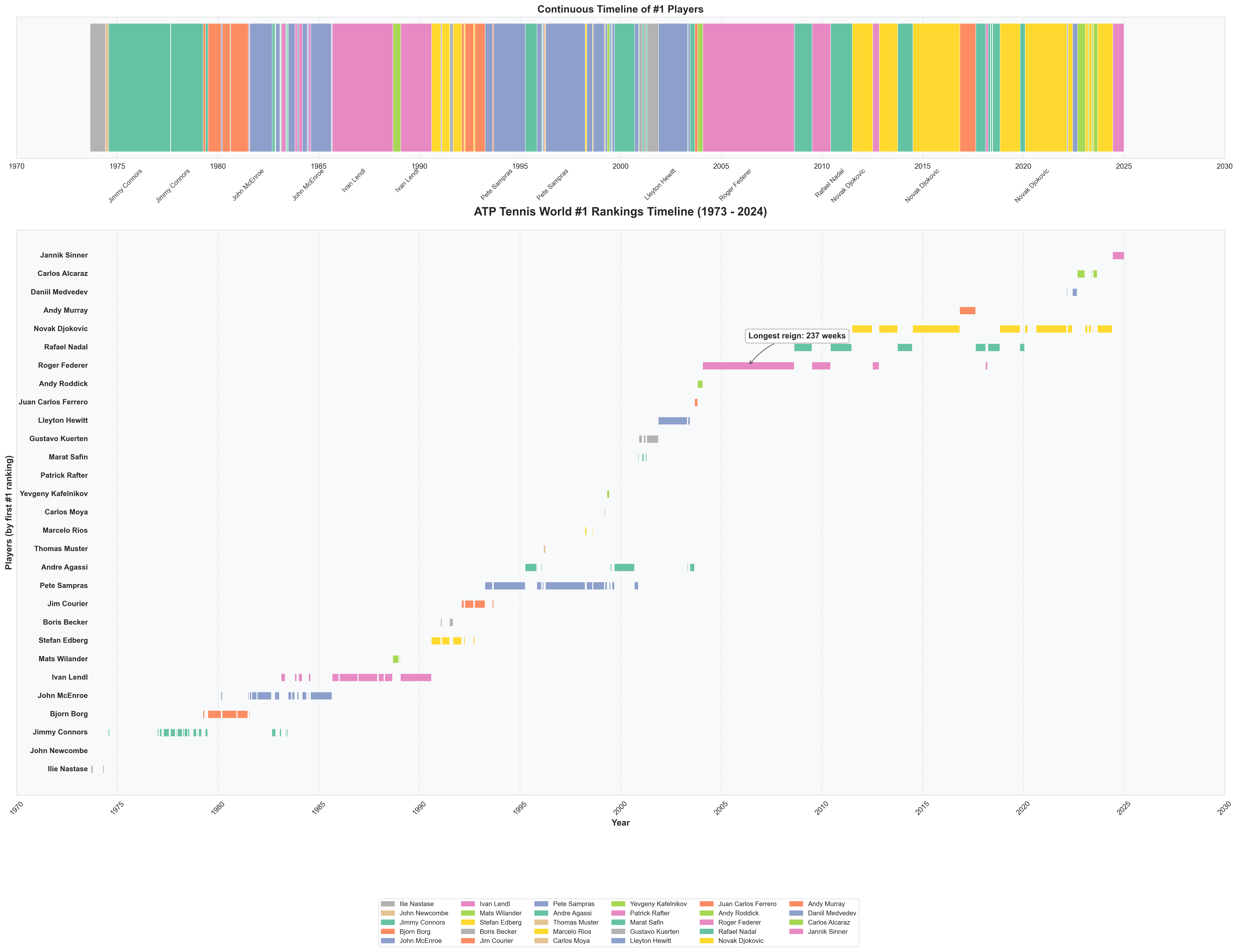
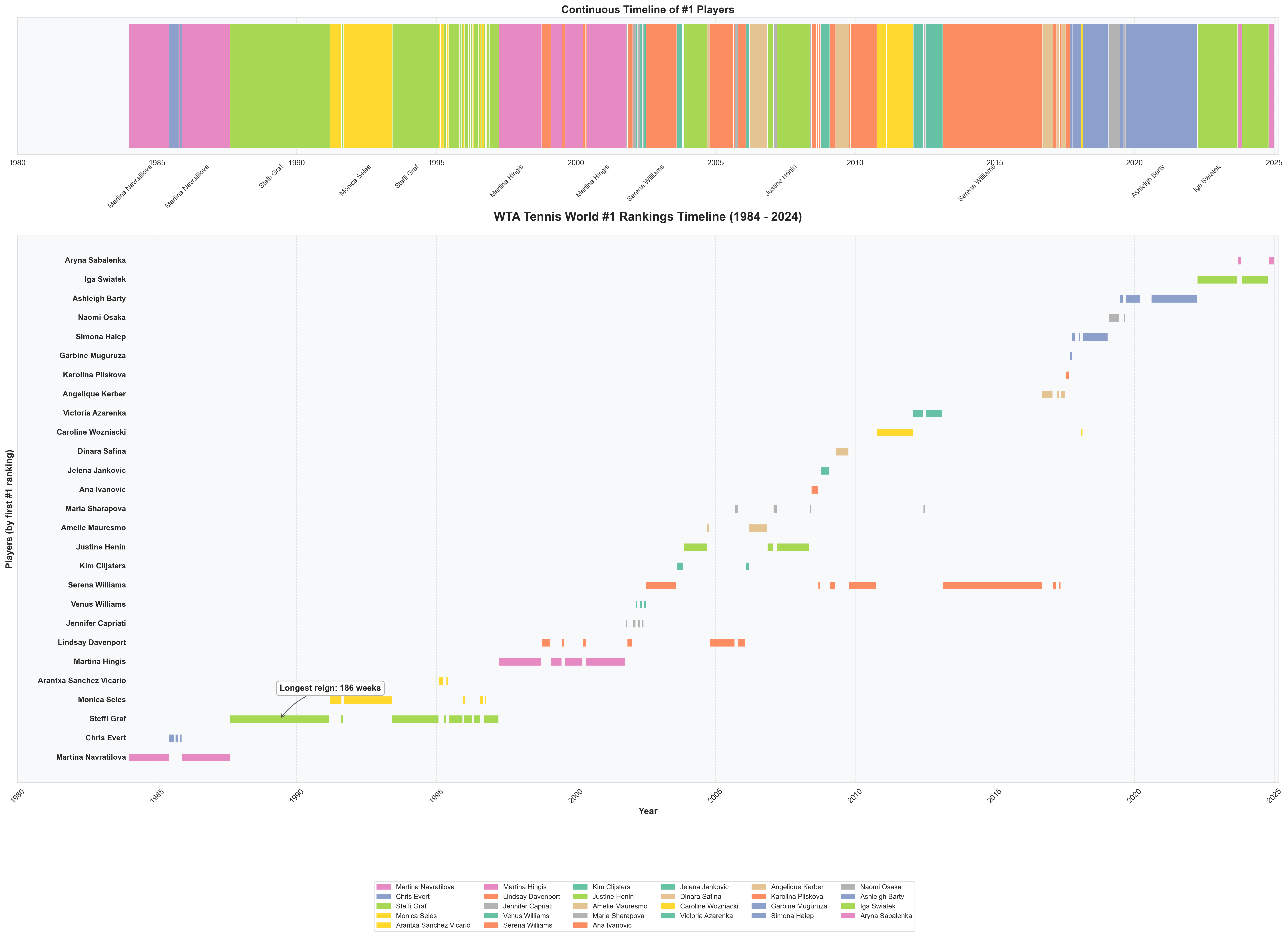
Player Rank History

I was intrigued when I saw that Sackmann also had player rank history week over week. There’s more I want to do with the application to tennis-scorigami but for now, I thought it was fun to create some of these visualizations:

atp-number-one-timeline

ATP #1 Ranking Timeline

wta-number-one-timeline

WTA #1 Ranking Timeline

Conclusion

This was an awesome project to work on and I still think there’s a ton we could do here. If you find any data quality issues, please reach out. Some thoughts about where we could take this:

Richer match data leading -> embeddings -> vector search
WebRTC for real time collaboration in some way
Popularity of searches
More exposure of conditional probabilities given a player and a score, what might happen next
- Perhaps leverage this into some type of betting.

As always, feel free to reach out with any questions.

Tennis Scorigami

Tennis Scorigami

Table of Contents

Motivation

More Specific Motivation

Demo

Features

Challenges

Data Consolidation

Being Cheap

Fetching 108k Nodes

Rendering 108k Nodes

2D Sigma Graph

3D Force Graph

Streaming + NDJSON

Unfurl Previews

Surprises

The counting

Why only ~8 % have shown up on court

Tech Stack

Engineering + Design

Other Fun Visualizations

Player Rank History

Conclusion