
✍️ Motivating Visualizations
Today, we’re going to learn how to teach a computer to write. I don’t mean generating text (which would have been probably a better thing to study in college), I mean learning to write like a human learns how to write with a pen and paper. My results (eventually) were pretty good, here are some motivating visualizations.
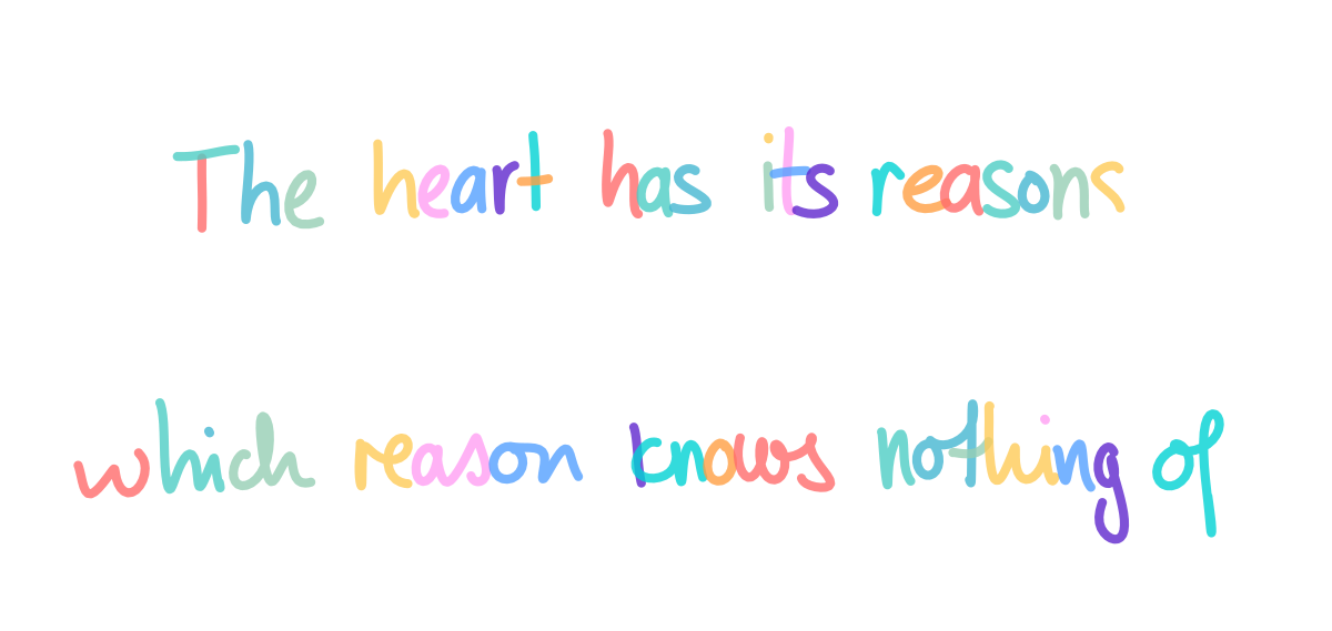
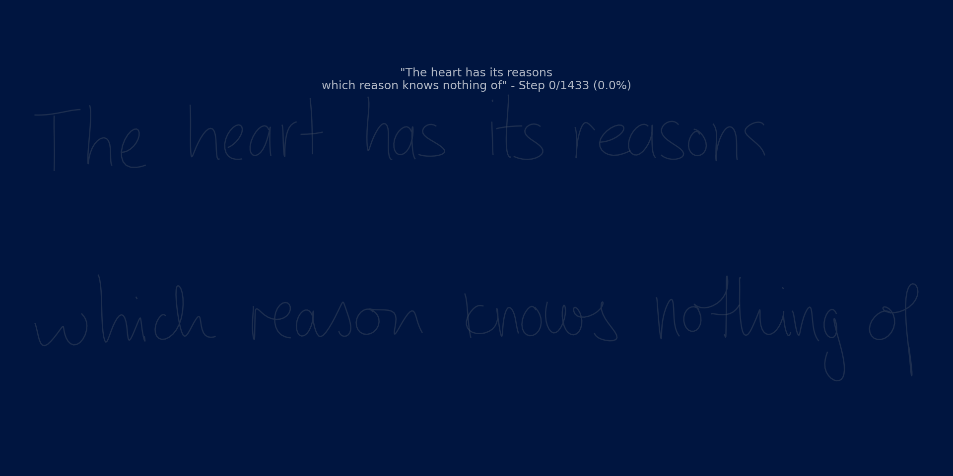
Let’s look at one. My family used to have this hung over our kitchen sink when I was a kid. I ate breakfast every day looking at it.
The heart has its reasons which reason knows nothing of
, "Pensées"

Again, I’d recommend jumping down to here: Synthesis Model Sampling. Arguably, the best part of this post. I’ll discuss what all these visualizations mean in detail.
This is a relatively long post! I would encourage you if you're trying to learn from 0 -> 1 to read the whole thing, but feel free to jump around as you so wish. I would say there's three main portions: concept, theory, and code.
My purpose here was to build up from the basics and really understand the flow. I provide quite a couple of models so we can see the progression from a simple neural net to a basic LSTM to Peephole LSTM to a stacked cascade of Peephole LSTMs to Mixture Density Networks to Attention Mechanism to Attention RNN to the Handwriting Prediction Network to finally throwing it all together to the full Handwriting Synthesis Network that Graves originally wrote about.
There's other things that maybe I'll discuss in the future like the need to pickle JAX models because if they're XLA compatible then you can't run inference on your CPU and issues like that. Another thing I didn't discuss really was temperature and bias for sampling. I also (sadly) didn't cover priming. However, I spent far more time on this than I should have. If you have any questions - as always - feel free to reach out if curious.
Enjoy!
One thing that I would highly recommend - if you're interested in the theory of LSTMs and why sigmoid vs tanh activations were chosen, I would really encourage reading Chris Olah's Understanding LSTMs blog post. It does a fantastic job.
🥅 Motivation
This motivation is clear - this is something that I have wanted to find the time to do right since college. My engineering thesis was on this Graves paper. My senior year, I worked with my good friend (also he’s a brilliant engineer) Tom Wilmots to understand and dive into this paper.
I’m going to pull pieces of that, but the time has changed, and I wanted to revisit some of the work we did, hopefully clean it up, and finally put a nail in this (so my girlfriend / friends don’t have to keep hearing about it).
👨🏫 History
Tom and I were very interested in the concept of teaching a computer how to write in college. There is a very famous paper that was published around 2013 from Canadian computer scientist Alex Graves, titled Generating Sequences With Recurrent Neural Networks. At Swarthmore, you have to do Engineering thesis, called E90s. It’s basically a year (although I’d argue it’s more of a semester when it all shakes out) long project focused on doing a piece of work you’re proud of.
Tom and My Engineering Thesis
For the actual paper that we wrote, check it out here:
You can also check it out here: Application of Neural Networks with Handwriting Samples.
🙏 Acknowledgements
Before I dive in, I do want to make some acknowledgements just given this is a partial resumption of work.
- Tom Wilmots - One of the brightest and best engineers I’ve worked with. He was an Engineering and Economics double major from Swarthmore. Pretty sure I would have failed my E90 thesis without him.
- Matt Zucker - One of my role models and constant inspirations, Matt was kind enough to be Tom and my academic advisor for this final engineering project. He is the best professor I’ve come across.
- Alex Graves - A professor that both Tom and I had the pleasure of working with. He responded to our emails, which I’m still very appreciative of. You can see more about his work at the University of Toronto here). He is the author of this paper, which Matt found for us and pretty much was the basis of our project. He’s also the creator of the Neural Turing Machine, which peaked my interest after having taken Theory of Computation, with my other fantastic professor Lila Fontes and learning about Turing machines.
- David Ha - Another brilliant scientist who we had the privilege of corresponding with. Check out his blog here. It’s beautiful. He also is very prolific on ArXiv which is always cool to see.
📝 Concept
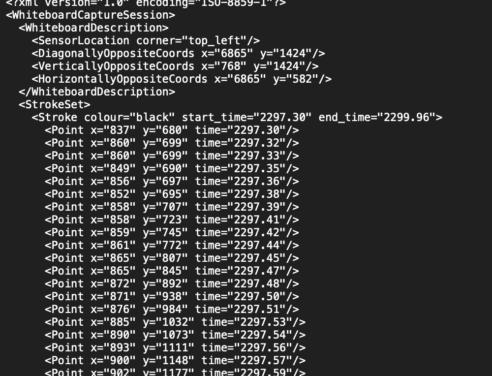
This section is going to be for non-technical people to understand what we were trying to do. It’s relatively simple. At a very high level, we are trying to teach a computer how to generate human looking handwriting. To do that, we are going to train a neural network. We are going to use a public dataset, called IAM Online Handwriting Database. This dataset had a ton of people write on a tablet where the data was being recorded. It collected basically sets of Stroke data, which were tuples of $(x, y, t)$, where $(x, y)$ are the coordinates on the tablet, and $t$ is the timestamp. We’ll use this data to train a model so that across all of the participants we have this blended approach of how to write like a human.
👾 Software
In college, we decided between Tensorflow and Pytorch. In college, we used Tensorflow. However, given the times, I wanted to still resume our tensorflow approach with updated designs, but I also wanted to try and use JAX. JAX is… newer. But it’s gotten some hype online and I think there’s a solid amount of adoption across the bigger AI labs now. In my opinion, Tensorflow is dying, Pytorch is the new status quo, and JAX is the new kid on the block. However, I’m not an ML researcher clearing millions of dollars. So grain of salt. This clickbaity article which declares “Pytorch is dead. Long live JAX” got a ton of flak online, but regardless… it piqued my interest enough to try it here.
I’ll cover all three here and yeah probably dive deepest into tensorflow… but feel free to skip this section.
Tensorflow
Programming Paradigm
Tensorflow has this interesting programming paradigm, where you are more or less creating a graph. You define Tensors and then when you run your dependency graph, those things are actually translated.
I have this quote from the Tensorflow API:
There’s only two things that go into Tensorflow.
- Building your computational dependency graph.
- Running your dependency graph.
This was the old way, but now that’s not totally true. Apparently, Tensorflow 2.0 helped out a lot with the computational model and the notion of eagerly executing, rather than building the graph and then having everything run at once.
Versions - How the times have changed
So - another fun fact - when we were doing this in college, we were on tensorflow version v0.11!!! They hadn’t even released a major version. Now, I’m doing this on Tensorflow 2.16.1. So the times have definitely changed.

Definitely haven’t been able to keep up with all those changes.
Tensorboard
Another cool thing about Tensorflow that should be mentioned is the ability to utilize the Tensorboard. This is a visualization suite that creates a local website where you can interactively and with a live stream visualize your dependency graph. You can do cool things like confirm that the error is actually decreasing over the epochs.
We used this a bit more in college. I didn’t get a real chance to dive into the updates made from this.
Pytorch
PyTorch is now basically the defacto standard for most serious research labs and AI shops. To me, it seems like things are still somewhat ported to Tensorflow for production, but I’m not totally sure about convention.
Pytorch seems to thread the line between Tensorflow and JAX. Functions don’t necessarily need to be pure to be utilized. You can loop and mutate state in a nn.Module just fine.
I won’t be covering pytorch but I certainly will come back around to it in later projects.
JAX
The new up and comer! I think it’s largely a crowd favorite for it’s speed. Documentation is obviously worse. One Redditor summarized it nicely:
Comment
byu/Few-Pomegranate4369 from discussion
inMachineLearning
I hit numerous roadblocks where functions weren’t actually pure and then the JIT compile portion basically failed on startup.
Programming Paradigm
JAX and Pytorch are definitely the most like traditional Python imperative flow. The restriction on JAX is largely around pure functions. Tensorflow is also gradually moving away from the compile your graph and then run it paradigm.
📊 Data
We’re using the IAM Online Handwriting Database. Specifically, I’m looking at data/lineStrokes-all.tar.gz, which is XML data that looks like this:
There’s also this note:
The database is divided into 4 parts, a training set, a first validation set, a second validation set and a final test set. The training set may be used for training the recognition system, while the two validation sets may be used for optimizing some meta-parameters. The final test set must be left unseen until the final test is performed. Note that you are allowed to use also other data for training etc, but report all the changes when you publish your experimental results and let the test set unchanged (It contains 3859 sequences, i.e. XML-files - one for each text line).
So that determines our training set, validation set, second validation set, and a final test set.
🧠 Base Neural Network Theory
I am not going to dive into details as much as we did for our senior E90 thesis, but I do want to cover a couple of the building blocks.
Lions, Bears, and Many Neural Networks, oh my
I would highly encourage you to check out this website: https://www.asimovinstitute.org/neural-network-zoo/. I remember seeing it in college when working on this thesis and was stunned. If you’re too lazy to click, check out the fun picture:
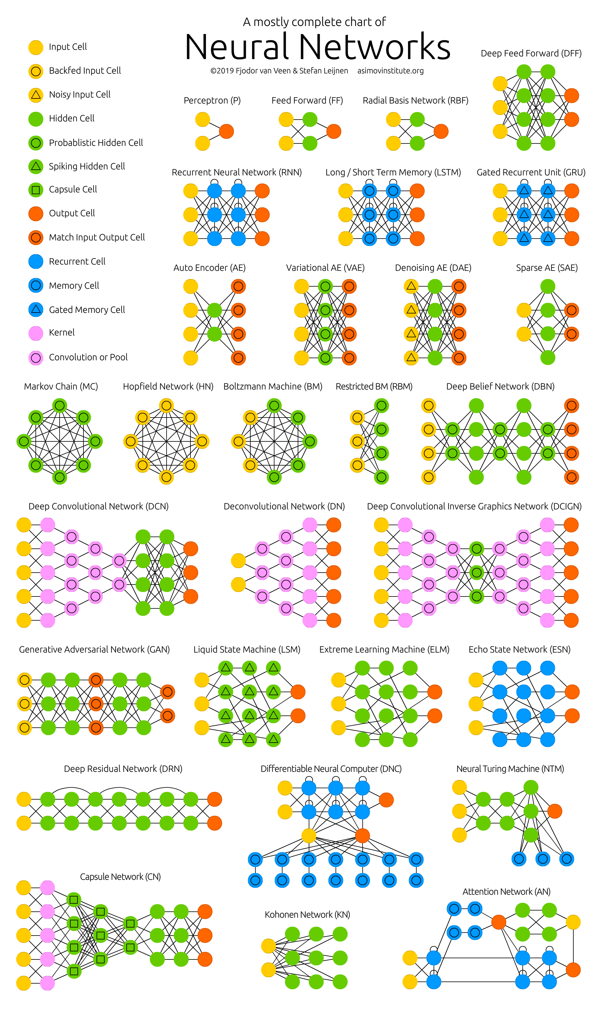
We’re going to explore some of the zoo in a bit more detail, specifically, focusing on LSTMs.
Basic Neural Network

The core structure of a neural network is the connections between all of the neurons. Each connection carries an activation signal of varying strength. If the incoming signal to a neuron is strong enough, then the signal is permeated through the next stages of the network.
There is a input layer that feeds the data into the hidden layer. The outputs from the hidden layer are then passed to the output layer. Every connection between nodes carries a weight determining the amount of information that gets passed through.
Hyper Parameters
For a basic neural network, there are generally three hyperparameters:
- pattern of connections between all neurons
- weights of connections between neurons
- activation functions of the neurons
In our project however, we focus on a specific class of neural networks called Recurrent Neural Networks (RNNs), and the more specific variation of RNNs called Long Short Term Memory networks (LSTMs).
However, let’s give a bit more context. There’s really two broad types of neural networks:
Feedforward Neural Network
These neural networks channel information in one direction.
The figure above is showing a feedforward neural network because the connections do not allow for the same input data to be seen multiple times by the same node.
These networks are generally very well used for mapping raw data to categories. For example, classifying a face from an image.
Every node outputs a numerical value that it then passes to all its successor nodes. In other words:
\[\begin{align} y_j = f(x_j) \end{align} \tag{1}\]where
\[\begin{align} x_j = \sum_{i \in P_j} w_{ij} y_i \end{align} \tag{2}\]where
- $y_j$ is the output of node $j$
- $x_j$ is the total weighted input for node $j$
- $w_{ij}$ is the weight from node $i$ to node $j$
- $y_i$ is the output from node $i$
- $P_j$ represents the set of predecessor nodes to node $j$
Also note, $f(x)$ should be a smooth non-linear activation function that maps outputs to a reasonable domain. Some common activation functions include $\tanh(x)$ or the sigmoid function. These complex functions are necessary because the neural network is literally trying to learn a non-linear pattern.
Backpropagation
Backpropagation is the mechanism in which we pass the error back through the network starting at the output node. Generally, we minimize using [stochastic gradient descent][stoch-grad-desc]. Again, lots of different ways we can define our error, but we can use sum of squared residuals between our $k$ targets and the output of $k$ nodes of the network.
\[\begin{align} E = \frac{1}{2} \sum_{k}(t_k - y_k)^2 \end{align} \tag{3}\]The gradient descent part comes in next. We generate the set of all gradients with respect to error and minimize these gradients. We’re minimizing this:
\[\begin{align} g_{ij} = - \frac{\delta E}{\delta w_{ij}} \end{align} \tag{4}\]So overall, we’re continually altering the weights and minimizing their individual effect oin the overall error of the outputs.
The major downfall of this simple network is that we don’t have full context. With sequences, there’s not enough information about the previous words, so the context is missing. And that leads us to our next structure.
Recurrent Neural Network
Recurrent Neural Networks (RNNs) have a capacity to remember. This memory stems from the fact that their input is not only the current input vector but also a variation of what they output at previous time steps.
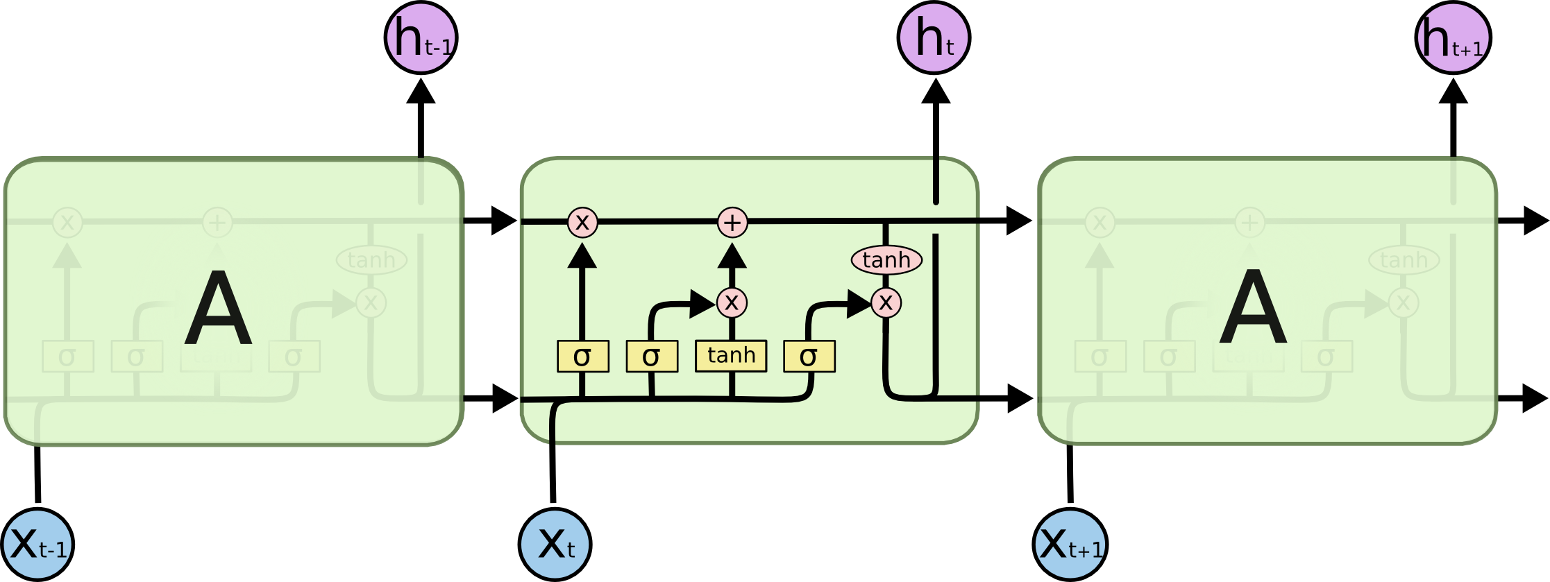
This visualization from Christopher Olah (who holy hell i just realized is a co-founder of Anthropic, but who Tom and I used to follow closely in college) is a great visualization:
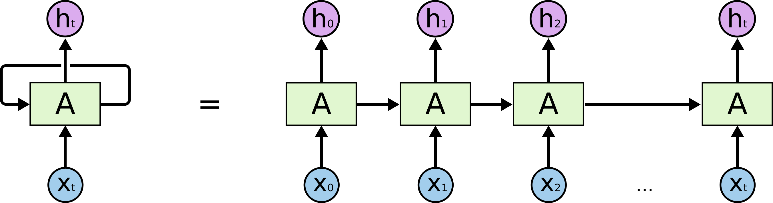
This RNN module is being unrolled over multiple timestamps. Information is passed within a module at time step $t$ to the module at $t+1$.
Per Tom and my paper,
An ideal RNN would theoretically be able to remember as far back as was necessary in order to to make an accurate prediction. However, as with many things, the theory does not carry over to reality. RNNs have trouble learning long term dependencies due to the vanishing gradient problem. An example of such a long term dependency might be if we are trying to predict the last word in the following sentence ”My family originally comes from Belgium so my native language is PREDICTION”. A normal RNN would possibly be able to recognize that the prediction should be a language but it would need the earlier context of Belgium to be able to accurately predict DUTCH.
Topically, this is why the craze around LLMs is so impressive. There’s a lot more going on with LLMs… which… I will not cover here.
The notion of backpropagation is basically the same just we also have the added dimension of time.
The crux of the issue is that RNNs have many layers and as we begin to push the derivatives to zero. The gradients become too small and cause underflow. In actual meaning, the networks then cease to be able to learn.
However, Sepp Hochreiter and Juergen Schmidhuber developed the Long Short Term Memory (LSTM) unit that solved this vanishing gradient problem.
Long Short Term Memory Networks
Long Short Term Memory (LSTM) networks are specifically designed to learn long term dependencies.
Every form of RNN has repeating modules that pass information across timesteps, and LSTMs are no different. Where they different is the inner structure of each module. While a standard RNN might have a single neural layer, LSTMs have four.
Understanding the LLM Structure
So let’s better understand the structure above. There’s a way more comprehensive walkthrough here. I’d encourage you to check out that walkthrough.
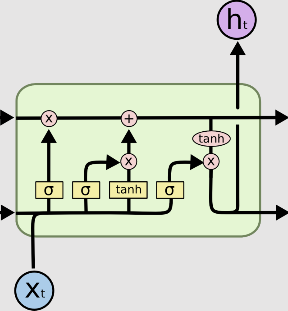
The top line is key to the LSTM’s ability to remember. It is called the cell state. We’ll reference it as $C_t$.
The first neural network layer is a sigmoid function. It takes as input the concatenation between the current input $x_t$ and the output of the previous module $h_{t-1}$. This is coined as the forget gate. It is in control of what to forget for the cell state. The sigmoid function is a good architecture decision here because it basically outputs numbers between [0,1] indicating how much the layer should let through.
We piecewise multiply the output of the sigmoid layer $f_t = \sigma(W_f \cdot [h_{t-1}, x_t] + b_f)$, with the cell state from the previous module $C_{t-1}$, forgetting the things that it doesn’t see as important.
Then right in the center of the image above there are two neural network layers which make up the update gate. First, $x_t \cdot h_{t-1}$ is pushed through both a sigmoid ($\sigma$) layer and a $\tanh$ layer. The output of this sigmoid layer $i_t = \sigma (W_i \cdot [h_{t-1}, x_t] + b_C)$ determines which values to use to update, and the output of the $\tanh$ layer $\hat{C} = \sigma (W_C \cdot [h_{t-1}, x_{t} + b_C$, proposes an entirely new cell state. These two results are then piecewise multiplied and added to the current cell state (which we just edited using the forget layer) outputting the new cell state $C_t$.
The final neural network layer is called the output gate. It determines the relevant portion of the cell state to output as $h_t$. Once again, we feed $x_t \cdot h_{t-1}$ through a sigmoid layer whose output, $o_t = \sigma (W_o \cdot [h_{t-1}, x_t] + b_o)$, we piecewise multiple with $\tanh(C_t)$. The result of the multiplication determines the output of the LSTM module. Note that the purple $\tanh$ is not a neural network layer, but a piecewise multiplication intended to push the current cell state into a reasonable domain.
I'm serious... you guys should check out Olah's Understanding LSTMs. Here he is back in 2015 strongly foreshadowing transformers given the focus on attention (which is truly the hardest part of all this) blog post.
🧬 Concepts to Code
When very first starting this project, I kind of figured that I would be able to use some of my college code, but looking back. It’s quite a mess and I don’t think that’s the way to go about it.
I thought for awhile about how best to structure this part. Meaning the code, but also how to show this in my blog post. With all the buzz about JAX, I wanted to try that too, so I thought it’d be helpful to show a side be side translation of the tensorflow vs jax code. My hope is that we’ll walk through the concepts and have a good understanding of the theory, and then the code will make a bit more sense. One note, is that I was a bit burnt of this project by the end so the JAX code I was trying to use optax (link) and flax (link) as much as possible to cut down on bulkiness of code.
So we’ll walk through the building blocks (in terms of code) and then show the code translations.
LSTM Cell with Peephole Connections
Theory
The basic LSTM cell (tf.keras.layers.LSTMCell) does not actually have the notion of peephole connections.
According to the very functional code that sjvasquez wrote, I don’t think we actually need it, but I figured it would be fun to implement regardless. Back in the old days, when Tensorflow would support add-ons, there was some work around this here, but that project was deprecated.
That being said…. the JAX / Flax code also doesn’t have LSTMs out of the gate with peepholes and so…. I just used the normal ones. The JAX model actually trained a bit better, but I think part of that was also just patience.
Code
def call(self, inputs: tf.Tensor, state: Tuple[tf.Tensor, tf.Tensor]):
    """
    This is basically implementing Graves's equations on page 5
    https://www.cs.toronto.edu/~graves/preprint.pdf
    equations 5-11.

    From the paper,
    * sigma is the logistic sigmoid function
    * i -> input gate
    * f -> forget gate
    * o -> output gate
    * c -> cell state
    * W_{hi} - hidden-input gate matrix
    * W_{xo} - input-output gate matrix
    * W_{ci} - are diagonal
        + so element m in each gate vector only receives input from
        + element m of the cell vector
    """

    # going to be shape (?, num_lstm_units)
    h_tm1, c_tm1 = state

    # basically the meat of eq, 7, 8, 9, 10
    z = tf.matmul(inputs, self.kernel) + tf.matmul(h_tm1, self.recurrent_kernel) + self.bias
    i_lin, f_lin, g_lin, o_lin = tf.split(z, num_or_size_splits=4, axis=1)

    if self.should_apply_peephole:
        pw_i = tf.expand_dims(self.peephole_weights[:, 0], axis=0)
        pw_f = tf.expand_dims(self.peephole_weights[:, 1], axis=0)
        i_lin = i_lin + c_tm1 * pw_i
        f_lin = f_lin + c_tm1 * pw_f

    # apply activation functions! see Olah's blog
    i = tf.sigmoid(i_lin)
    f = tf.sigmoid(f_lin)
    g = tf.tanh(g_lin)
    c = f * c_tm1 + i * g

    if self.should_apply_peephole:
        pw_o = tf.expand_dims(self.peephole_weights[:, 2], axis=0)
        o_lin = o_lin + c * pw_o

    o = tf.sigmoid(o_lin)

    # final hidden state -> eq. 11
    h = o * tf.tanh(c)
    return h, [h, c]
class HandwritingModel(nnx.Module):
def __init__(
self,
config: ModelConfig,
rngs: nnx.Rngs,
synthesis_mode: bool = False,
) -> None:
self.config = config
self.synthesis_mode = synthesis_mode
# rngs is basically a set of random keys / number generators
self.lstm_cells = self._build_lstm_stack(rngs)
if synthesis_mode:
# i mean we really only care about synthesis mode, but in
# this case we can make it explicit that if we have it then we should add our
# attention layer
self.attention_layer = nnx.Linear(
config.hidden_size + config.alphabet_size + 3, 3 * config.num_attention_gaussians, rngs=rngs
)
# mdn portion
self.mdn_layer = self._build_mdn_head(rngs)
def _build_lstm_stack(self, rngs: nnx.Rngs):
cells = []
for i in range(self.config.num_layers):
if i == 0:
if self.synthesis_mode:
# so if we're in synthesis mode, then we need to add the alphabet size
# and the 3 dimensions of the input stroke
# that's because our alphabet size is the number of characters in our alphabet
# and the 3 dimensions of the input stroke are the x, y, and eos values
in_size = self.config.alphabet_size + 3
else:
in_size = 3
else:
# similar in both (just in synthesis we only care if we need to expand by the alphabet size)
in_size = self.config.hidden_size + 3
if self.synthesis_mode:
in_size += self.config.alphabet_size
# ok... being lazy but this is just standard LSTM
cells.append(
{"linear": nnx.Linear(in_size + self.config.hidden_size, 4 * self.config.hidden_size, rngs=rngs)}
)
return cells
def lstm_cell(
self, x: jnp.ndarray, h: jnp.ndarray, c: jnp.ndarray, layer_idx: int
) -> Tuple[jnp.ndarray, jnp.ndarray]:
# just think about this as grabbing the W and b for our matrix mults
linear = self.lstm_cells[layer_idx]["linear"]
combined = jnp.concatenate([x, h], axis=-1)
gates = linear(combined)
i, f, g, o = jnp.split(gates, 4, axis=-1)
# activations
i = nnx.sigmoid(i)
f = nnx.sigmoid(f)
g = nnx.tanh(g)
o = nnx.sigmoid(o)
# get new LSTM cell state
c_new = f * c + i * g
h_new = o * nnx.tanh(c_new)
return h_new, c_newGaussian Mixture Models
Theory
Gaussian Mixture Models are an unsupervised technique to learn an underlying probabilistic model.
Brilliant has an incredible explanation walking through the theory here. I’d encourage you to check it out, but at a very high level:
- A number of Gaussians is specified by the user
- The algo learns various parameters that represent the data while maximizing the likelihood of seeing such data
So if we have $k$ components, for a multivariate Gaussian mixture model, we’ll learn $k$ means, $k$ variances, $k$ mixture weights, $k$ correlations through expectation maximization.
From Brilliant, there are really two steps for the EM step:
The first step, known as the expectation step or E step, consists of calculating the expectation of the component assignments $C_k$ for each data point $x_i \in X$ given the model parameters $\phi_k, \mu_k$ , and $\sigma_k$ .
The second step is known as the maximization step or M step, which consists of maximizing the expectations calculated in the E step with respect to the model parameters. This step consists of updating the values $\phi_k, \mu_k$ , and $\sigma_k$ .
Code
There’s actually not a whole lot of code to provide here. GMMs are more of the technique that we’ll combine with the output of a neural network. That leads us smoothly to our next section.
Mixture Density Networks
Theory
Mixture Density Networks are an extension of GMMs that predict the parameters of a mixture probability distribution.

Per our paper:
The idea is relatively simple - we take the output from a neural network and parametrize the learned parameters of the GMM. The result is that we can infer probabilistic prediction from our learned parameters. If our neural network is reason- ably predicting where the next point might be, the GMM will then learn probabilistic parameters that model the distribution of the next point. This is different in a few key aspects. Namely, we now have target values because our data is sequential. Therefore, when we feed in our targets, we minimize the log likelihood based on those expectations, thus altering the GMM portion of the model to learn the predicted values.
More or less though, the problem we’re trying to solve is predicting the next input given our output vector. Essentially, we’re asking for $\text{Pr}(x_{t+1} | y_t)$. I’m not going to show the proof (we didn’t in our paper right), but the equation for the conditional probability is shown below:
\[\begin{align} \text{Pr}(x_{t+1} | y_t) = \sum_{j=1}^{M} \pi_{j}^t \mathcal{N} (x_{t+1} \mid \mu_j^t, \sigma_j^t, \rho_j^t) \end{align} \tag{5}\]where
\[\begin{align} \mathcal{N}(x \mid \mu, \sigma, \rho) = \frac{1}{2\pi \sigma_1 \sigma_2 \sqrt[]{1-\rho^2}} \exp \left[\frac{-Z}{2(1-\rho^2)}\right] \end{align} \tag{6}\]and
\[\begin{align} Z = \frac{(x_1 - \mu_1)^2 }{\sigma_1^2} + \frac{(x_2 - \mu_2)^2}{\sigma_2^2} - \frac{2\rho (x_1 - \mu_1) (x_2 - \mu_2) }{\sigma_1 \sigma_2} \end{align} \tag{7}\]Now, there’s a slight variation here because we have a handwriting specific end-of-stroke parameter. So we modify our conditional probability formula to result in our final calculation of:
\[\begin{align} \textrm{Pr}(x_{t+1} \mid y_t ) = \sum\limits_{j=1}\limits^{M} \pi_j^t \; \mathcal{N} (x_{t+1} \mid \mu_j^t, \sigma_j^t, \rho_j^t) \begin{cases} e_t & \textrm{if } (x_{t+1})_3 = 1 \\ 1-e_t & \textrm{otherwise} \end{cases} \end{align} \tag{8}\]And that’s it! That’s our final probability output from the MDN. Once we have this, performing our expectation maximization is simple as our loss function that we choose to minimize is just:
\[\begin{align} \mathcal{L}(\mathbf{x}) = - \sum\limits_{t=1}^{T} \log \textrm{Pr}(x_{t+1} \mid y_t) \end{align} \tag{9}\]Code
Here’s the corresponding code section for my mixture density network.
class MixtureDensityLayer(tf.keras.layers.Layer):
    def __init__(
        self,
        num_components,
        name="mdn",
        temperature=1.0,
        enable_regularization=False,
        sigma_reg_weight=0.01,
        rho_reg_weight=0.01,
        entropy_reg_weight=0.1,
        **kwargs,
    ):
        super(MixtureDensityLayer, self).__init__(name=name, **kwargs)
        self.num_components = num_components
        # The number of parameters per mixture component: 2 means, 2 standard deviations, 1 correlation, 1 weight , 1 for eos
        # so that's our constant num_mixture_components_per_component
        self.output_dim = num_components * NUM_MIXTURE_COMPONENTS_PER_COMPONENT + 1
        self.mod_name = name
        self.temperature = temperature
        self.enable_regularization = enable_regularization
        self.sigma_reg_weight = sigma_reg_weight
        self.rho_reg_weight = rho_reg_weight
        self.entropy_reg_weight = entropy_reg_weight

    def build(self, input_shape):
        graves_initializer = tf.keras.initializers.TruncatedNormal(mean=0.0, stddev=0.075)

        self.input_units = input_shape[-1]
        # weights
        # lots of weight initialization here... could simplify here too

        # biases
        # lots of bias initialization here... could simplify this part by just doing a massive
        # and splitting... see the code if you're curious
        super().build(input_shape)

    def call(self, inputs, training=None):
        temperature = 1.0 if not training else self.temperature

        pi_logits = tf.matmul(inputs, self.W_pi) + self.b_pi
        pi = tf.nn.softmax(pi_logits / temperature, axis=-1)  # [B, T, K]
        # clipping here... I was getting cooked by NaN creep
        pi = tf.clip_by_value(pi, 1e-6, 1.0)

        mu = tf.matmul(inputs, self.W_mu) + self.b_mu  # [B, T, 2K]
        mu1, mu2 = tf.split(mu, 2, axis=2)

        log_sigma = tf.matmul(inputs, self.W_sigma) + self.b_sigma  # [B, T, 2K]
        # again, this might be overkill but seems realistic for clipping
        log_sigma = tf.clip_by_value(log_sigma, -5.0, 2.0)
        sigma = tf.exp(log_sigma)
        sigma1, sigma2 = tf.split(sigma, 2, axis=2)

        rho_raw = tf.matmul(inputs, self.W_rho) + self.b_rho
        rho = tf.tanh(rho_raw) * 0.9

        eos_logit = tf.matmul(inputs, self.W_eos) + self.b_eos

        return tf.concat([pi, mu1, mu2, sigma1, sigma2, rho, eos_logit], axis=2)
class HandwritingModel(nnx.Module):
def __init__(
self,
config: ModelConfig,
rngs: nnx.Rngs,
synthesis_mode: bool = False,
) -> None:
self.config = config
self.synthesis_mode = synthesis_mode
# rngs is basically a set of random keys / number generators
self.lstm_cells = self._build_lstm_stack(rngs)
if synthesis_mode:
# i mean we really only care about synthesis mode, but in
# this case we can make it explicit that if we have it then we should add our
# attention layer
self.attention_layer = nnx.Linear(
config.hidden_size + config.alphabet_size + 3, 3 * config.num_attention_gaussians, rngs=rngs
)
# mdn portion
self.mdn_layer = self._build_mdn_head(rngs)
#....
def __call__(
self,
inputs: jnp.ndarray,
char_seq: Optional[jnp.ndarray] = None,
char_lens: Optional[jnp.ndarray] = None,
initial_state: Optional[RNNState] = None,
return_state: bool = False,
) -> jnp.ndarray:
batch_size, seq_len, _ = inputs.shape
if initial_state is None:
h = jnp.zeros((self.config.num_layers, batch_size, self.config.hidden_size), inputs.dtype)
c = jnp.zeros_like(h)
kappa = jnp.zeros((batch_size, self.config.num_attention_gaussians), inputs.dtype)
window = jnp.zeros((batch_size, self.config.alphabet_size), inputs.dtype)
else:
h, c = initial_state.hidden, initial_state.cell
kappa, window = initial_state.kappa, initial_state.window
def step(carry, x_t):
h, c, kappa, window = carry
h_layers = []
c_layers = []
# layer1
if self.synthesis_mode:
layer1_input = jnp.concatenate([window, x_t], axis=-1)
else:
layer1_input = x_t
h1, c1 = self.lstm_cell(layer1_input, h[0], c[0], 0)
h_layers.append(h1)
c_layers.append(c1)
# layer1 -> attention
if self.synthesis_mode and char_seq is not None and char_lens is not None:
window, kappa = self.compute_attention(h1, kappa, window, x_t, char_seq, char_lens)
# attention -> layer2 and layer3
for layer_idx in range(1, self.config.num_layers):
if self.synthesis_mode:
layer_input = jnp.concatenate([x_t, h_layers[-1], window], axis=-1)
else:
layer_input = jnp.concatenate([x_t, h_layers[-1]], axis=-1)
h_new, c_new = self.lstm_cell(layer_input, h[layer_idx], c[layer_idx], layer_idx)
h_layers.append(h_new)
c_layers.append(c_new)
h_new = jnp.stack(h_layers)
c_new = jnp.stack(c_layers)
# mdn output from final hidden state
mdn_out = self.mdn_layer(h_layers[-1]) # [B, 6M+1]
return (h_new, c_new, kappa, window), mdn_out
# this was the major unlock for JAX performance
# it allows us to vectorize the computation over the time dimension
# transpose inputs from [B, T, 3] to [T, B, 3] for scan
inputs_transposed = inputs.swapaxes(0, 1)
(h, c, kappa, window), outputs = jax.lax.scan(step, (h, c, kappa, window), inputs_transposed)
# transpose back
outputs = outputs.swapaxes(0, 1)
if return_state:
final_state = RNNState(hidden=h, cell=c, kappa=kappa, window=window)
return outputs, final_state
return outputsMixture Density Loss
Theory
I already covered the theory above, so I won’t go into that here, but just figured it was easier to split out the code between network and calculating our loss. Note, there’s some pretty aggressive clipping going on just given I had some pretty high instability with JAX. I think partially because of the implementation and clipping but loss would just go to 0 rather than the program crashing. To be clear, loss going to zero was not desired.
Code
@tf.keras.utils.register_keras_serializable()
def mdn_loss(y_true, y_pred, stroke_lengths, num_components, eps=1e-8):
    """
    Mixture density negative log-likelihood computed fully in log-space.

    y_true: [B, T, 3]  -> (x, y, eos ∈ {0,1})
    y_pred: [B, T, 6*K + 1] -> (pi, mu1, mu2, sigma1, sigma2, rho, eos_logit)

    The log space change was because I was getting absolutely torched by the
    gradients when using the normal space.
    """
    out_pi, mu1, mu2, sigma1, sigma2, rho, eos_logits = tf.split(
        y_pred,
        [num_components] * 6 + [1],
        axis=2,
    )

    x, y, eos_targets = tf.split(y_true, [1, 1, 1], axis=-1)

    sigma1 = tf.clip_by_value(sigma1, 1e-2, 10.0)
    sigma2 = tf.clip_by_value(sigma2, 1e-2, 10.0)
    rho = tf.clip_by_value(rho, -0.9, 0.9)
    out_pi = tf.clip_by_value(out_pi, eps, 1.0)

    log_2pi = tf.constant(np.log(2.0 * np.pi), dtype=y_pred.dtype)
    one_minus_rho2 = tf.clip_by_value(1.0 - tf.square(rho), eps, 2.0)
    log_one_minus_rho2 = tf.math.log(one_minus_rho2)
    z1 = (x - mu1) / sigma1
    z2 = (y - mu2) / sigma2

    quad = tf.square(z1) + tf.square(z2) - 2.0 * rho * z1 * z2
    quad = tf.clip_by_value(quad, 0.0, 100.0)
    log_norm = -(log_2pi + tf.math.log(sigma1) + tf.math.log(sigma2) + 0.5 * log_one_minus_rho2)
    log_gauss = log_norm - 0.5 * quad / one_minus_rho2  # [B, T, K]

    # log mixture via log-sum-exp
    log_pi = tf.math.log(out_pi)  # [B, T, K]
    log_gmm = tf.reduce_logsumexp(log_pi + log_gauss, axis=-1)  # [B, T]

    # bce (bernoulli cross entropy) to help out with stability
    eos_nll = tf.nn.sigmoid_cross_entropy_with_logits(labels=eos_targets, logits=eos_logits)  # [B, T, 1]
    eos_nll = tf.squeeze(eos_nll, axis=-1)  # [B, T]

    nll = -log_gmm + eos_nll  # [B, T]
    if stroke_lengths is not None:
        mask = tf.sequence_mask(stroke_lengths, maxlen=tf.shape(y_true)[1], dtype=nll.dtype)
        nll = nll * mask
        denom = tf.maximum(tf.reduce_sum(mask), 1.0)
        return tf.reduce_sum(nll) / denom

    return tf.reduce_mean(nll)
def compute_loss(
predictions: jnp.ndarray,
targets: jnp.ndarray,
lengths: Optional[jnp.ndarray] = None,
num_mixtures: int = NUM_BIVARIATE_GAUSSIAN_MIXTURE_COMPONENTS,
) -> jnp.ndarray:
nc = num_mixtures
pi, mu1, mu2, s1, s2, rho, eos_pred = jnp.split(predictions, [nc, 2 * nc, 3 * nc, 4 * nc, 5 * nc, 6 * nc], axis=-1)
pi = nnx.softmax(pi, axis=-1)
s1 = jnp.exp(jnp.clip(s1, -10, 3))
s2 = jnp.exp(jnp.clip(s2, -10, 3))
rho = jnp.clip(nnx.tanh(rho) * 0.95, -0.95, 0.95)
eos_pred = jnp.clip(nnx.sigmoid(eos_pred), 1e-8, 1 - 1e-8)
x, y, eos = jnp.split(targets, [1, 2], axis=-1)
# major change is we compute log probabilities with better numerical stability
rho_sq = jnp.clip(rho**2, 0, 0.9025)
one_minus_rho_sq = jnp.maximum(1 - rho_sq, 1e-6)
norm = -jnp.log(2 * jnp.pi) - jnp.log(s1) - jnp.log(s2) - 0.5 * jnp.log(one_minus_rho_sq)
z1 = (x - mu1) / jnp.maximum(s1, 1e-6)
z2 = (y - mu2) / jnp.maximum(s2, 1e-6)
exp_term = -0.5 / one_minus_rho_sq * (z1**2 + z2**2 - 2 * rho * z1 * z2)
exp_term = jnp.clip(exp_term, -50, 0)
log_probs = norm + exp_term
log_pi = jnp.log(jnp.maximum(pi, 1e-8))
log_mixture = jax.nn.logsumexp(log_pi + log_probs, axis=-1)
eos_loss = -jnp.sum(eos * jnp.log(eos_pred) + (1 - eos) * jnp.log(1 - eos_pred), axis=-1)
loss = -log_mixture + eos_loss
loss = jnp.where(jnp.isnan(loss) | jnp.isinf(loss), 0.0, loss)
if lengths is not None:
mask = jnp.arange(predictions.shape[1]) < lengths[:, None]
loss = jnp.where(mask, loss, 0.0)
total_loss = jnp.sum(loss) / jnp.maximum(jnp.sum(mask), 1)
return jnp.where(jnp.isnan(total_loss) | jnp.isinf(total_loss), 0.0, total_loss)
mean_loss = jnp.mean(loss)
return jnp.where(jnp.isnan(mean_loss) | jnp.isinf(mean_loss), 0.0, mean_loss)Attention Mechanism
Theory
The attention mechanism really only comes into play with the Synthesis Network which sadly Tom and I never got to in college. The idea (similar to most attention notions) is that we need to tell our model more specifically where to focus. This isn’t like the transformer notion of attention from the famous “Attention is All You Need” paper, but it’s the idea that we have various Gaussians to indicate probabilistically where we should be focusing. We utilize one-hot encoding vectors over our input characters so that we can more clearly identify the numerical representation. So the question we’re basically answering is like “oh, i see a ‘w’ character, generally how far along do we need to write for that?” to help also answer the question of when do we need to terminate.
The mathematical representation is here:
Given a length $U$ character sequence $\mathbf{c}$ and a length $T$ data sequence $\mathbf{x}$, the soft window $w_t$ into $\mathbf{c}$ at timestep $t$ ($1 \leq t \leq T$) is defined by the following discrete convolution with a mixture of $K$ Gaussian functions
\[\begin{align} \phi(t, u) &= \sum_{k=1}^K \alpha^k_t\exp\left(-\beta_t^k\left(\kappa_t^k-u\right)^2\right)\\ w_t &= \sum_{u=1}^U \phi(t, u)c_u \end{align}\]where $\phi(t, u)$ is the \emph{window weight} of $c_u$ at timestep $t$.
Intuitively, the $\kappa_t$ parameters control the location of the window, the $\beta_t$ parameters control the width of the window and the $\alpha_t$ parameters control the importance of the window within the mixture.
The size of the soft window vectors is the same as the size of the character vectors $c_u$ (assuming a one-hot encoding, this will be the number of characters in the alphabet).
Note that the window mixture is not normalised and hence does not determine a probability distribution; however the window weight $\phi(t, u)$ can be loosely interpreted as the network’s belief that it is writing character $c_u$ at time $t$.
Code
@tf.keras.utils.register_keras_serializable()
class AttentionMechanism(tf.keras.layers.Layer):
    """
    Attention mechanism for the handwriting synthesis model.
    This is a version of the attention mechanism used in
    the original paper by Alex Graves. It uses a Gaussian
    window to focus on different parts of the character sequence
    at each time step.

    See section: 5.0 / 5.1
    """

    def __init__(self, num_gaussians, num_chars, name="attention", debug=False, **kwargs) -> None:
        super(AttentionMechanism, self).__init__(**kwargs)
        self.num_gaussians = num_gaussians
        self.num_chars = num_chars
        self.name_mod = name
        self.debug = debug

    def call(
        self,
        inputs,  # shape: [batch_size, num_gaussians, 3]
        prev_kappa,  # shape: [batch_size, num_gaussians]
        char_seq_one_hot,  # shape: [batch_size, char_len, num_chars]
        sequence_lengths,  # shape: [batch_size]
    ) -> tuple[tf.Tensor, tf.Tensor]:
        raw = tf.matmul(inputs, self.attention_kernel) + self.attention_bias
        alpha_hat, beta_hat, kappa_hat = tf.split(raw, 3, axis=1)  # shape: [batch_size, num_gaussians, 1]

        eps = tf.constant(1e-6, dtype=inputs.dtype)
        scaling = 0.1  # Gentler activation
        alpha = tf.nn.softplus(alpha_hat * scaling) + eps  # [B, G]
        beta = tf.nn.softplus(beta_hat * scaling) + eps  # [B, G]
        dkap = tf.nn.softplus(kappa_hat * scaling) + eps

        alpha = tf.clip_by_value(alpha, 0.01, 10.0)
        beta = tf.clip_by_value(beta, 0.01, 10.0)
        dkap = tf.clip_by_value(dkap, 1e-5, 0.5)

        kappa = prev_kappa + dkap
        kappa = tf.clip_by_value(kappa, 0.0, 30.0)

        char_len = tf.shape(char_seq_one_hot)[1]
        batch_size = tf.shape(inputs)[0]
        u = tf.cast(tf.range(1, char_len + 1), tf.float32)
        u = tf.reshape(u, [1, 1, -1])  # shape: [1, 1, char_len]
        u = tf.tile(u, [batch_size, self.num_gaussians, 1])  # shape: [batch_size, num_gaussians, char_len]

        alpha = tf.expand_dims(alpha, axis=-1)  # shape: [batch_size, num_gaussians, 1]
        beta = tf.expand_dims(beta, axis=-1)  # shape: [batch_size, num_gaussians, 1]
        kappa = tf.expand_dims(kappa, axis=-1)  # shape: [batch_size, num_gaussians, 1]

        exponent = -beta * tf.square(kappa - u)
        exponent = tf.clip_by_value(exponent, -50.0, 0.0)
        phi = alpha * tf.exp(exponent)  # shape: [batch_size, num_gaussians, char_len]
        phi = tf.reduce_sum(phi, axis=1)  # Sum over gaussians: [B, L]

        sequence_mask = tf.sequence_mask(sequence_lengths, maxlen=char_len, dtype=tf.float32)
        phi = phi * sequence_mask  # mask paddings

        phi = tf.where(tf.math.is_finite(phi), phi, tf.zeros_like(phi))
        # we don't normalize here - Graves calls that out specifically!
        # > Note that the window mixture is not normalised
        # > and hence does not determine a probability distribution; however the window
        # > weight φ(t,u) can be loosely interpreted as the network's belief that it is writ-
        # > ing character cu at time t.
        # still section 5.1

        # window vec
        phi = tf.expand_dims(phi, axis=-1)  # shape: [batch_size, char_len, 1]
        w = tf.reduce_sum(phi * char_seq_one_hot, axis=1)  # shape: [batch_size, num_chars]

        w = tf.where(tf.math.is_finite(w), w, tf.zeros_like(w))
        return w, kappa[:, :, 0]
def compute_attention(
self,
h: jnp.ndarray, # [B, H]
prev_kappa: jnp.ndarray, # [B, G]
window: jnp.ndarray, # [B, A]
x: jnp.ndarray, # [B, 3]
char_seq: jnp.ndarray, # [B, U, A] one-hot
char_lens: jnp.ndarray, # [B] lengths
) -> Tuple[jnp.ndarray, jnp.ndarray]:
"""Compute Gaussian window attention over character sequence."""
attention_input = jnp.concatenate([window, x, h], axis=-1)
params = self.attention_layer(attention_input) # [B, 3G]
params = nnx.softplus(params)
alpha, beta, kappa_inc = jnp.split(params, 3, axis=-1)
# again... probably sliiiiightly overkill
alpha = jnp.maximum(alpha, 1e-4)
beta = jnp.maximum(beta, 1e-4)
kappa_inc = jnp.maximum(kappa_inc, 1e-4)
# ok this was a trick from svasquez - the dividing by 25.0
# is to help kappa learn given that 25 is roughly the average
# number of strokes per sequence
kappa = prev_kappa + kappa_inc / 25.0
U = char_seq.shape[1]
positions = jnp.arange(U, dtype=jnp.float32)[None, None, :] # [1, 1, U]
kappa_exp = kappa[:, :, None] # [B, G, 1]
alpha_exp = alpha[:, :, None] # [B, G, 1]
beta_exp = beta[:, :, None] # [B, G, 1]
# gaussian window
phi = alpha_exp * jnp.exp(-beta_exp * (kappa_exp - positions) ** 2) # [B, G, U]
phi = jnp.sum(phi, axis=1)
# mask out positions beyond char_lens
mask = jnp.arange(U)[None, :] < char_lens[:, None] # [B, U]
phi = jnp.where(mask, phi, 0.0)
# so Graves said that
phi = phi / (jnp.sum(phi, axis=-1, keepdims=True) + 1e-8)
# Apply to character sequence
# window: [B, A] = sum_u phi[b,u]*char_seq[b,u,:]
window_new = jnp.einsum("bu,bua->ba", phi, char_seq)
return window_new, kappaStacked LSTM
Theory
The one distinction between Graves’s setup and a standard LSTM is that Graves uses a cascade of LSTMs. So we use the MDN to generate a probabilistic prediction however our neural network is the cascade of LSTMs.
Per our paper:
The LSTM cascade buys us a few different things. As Graves aptly points out, it mitigates the vanishing gradient problem even more greatly than a single LSTM could. This is because of the skip-connections. All hidden layers have access to the input and all hidden layers are also directly connected to the output node. As a result, there are less processing steps from the bottom of the network to the top.
So it looks something like this:
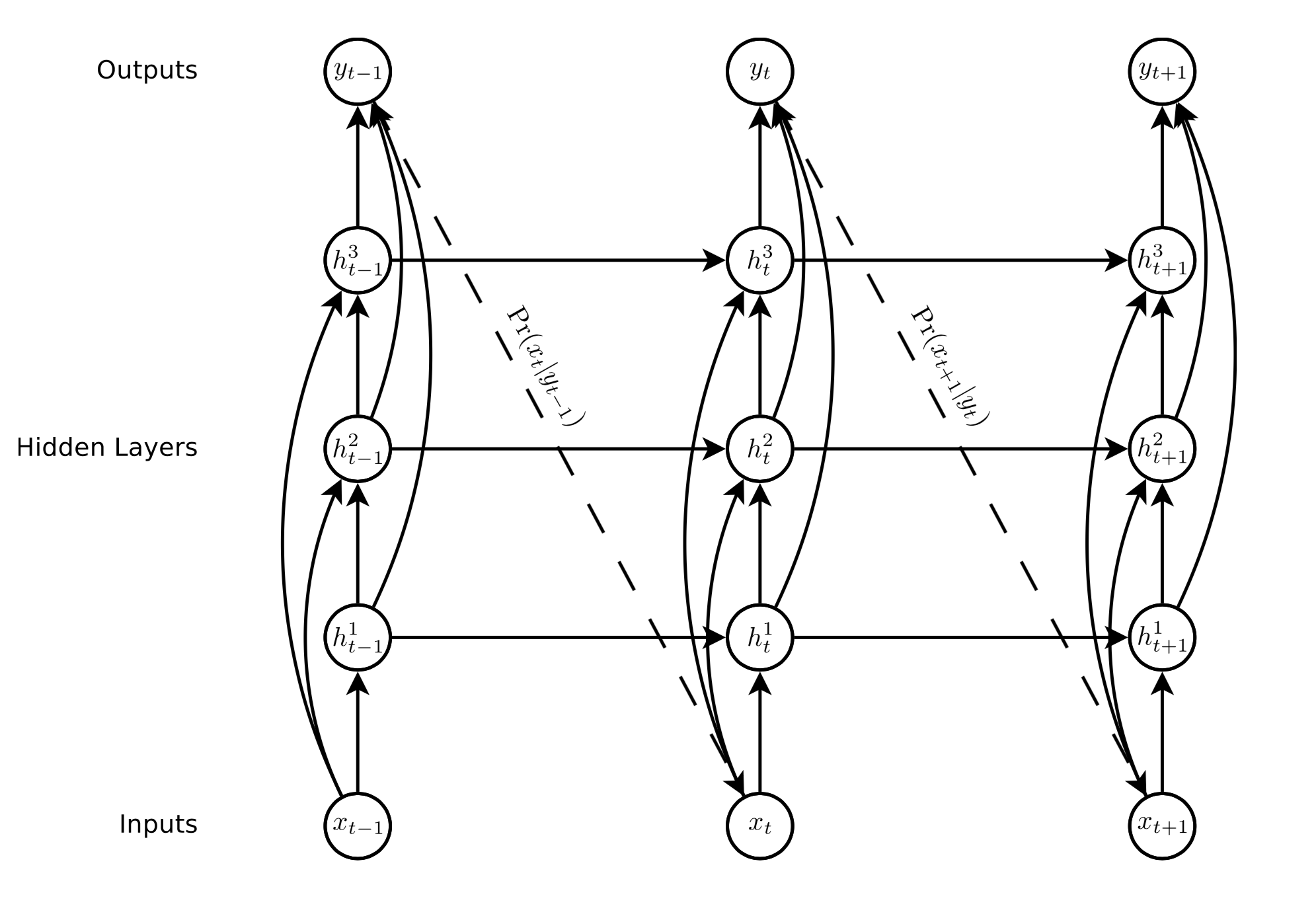
The one thing to note is that there is a dimensionality increase given we now have these hidden layers. Tom and I broke this down in our paper here:
Let’s observe the $x_{t-1}$ input. $h_{t-1}^1$ only has $x_{t-1}$ as its input which is in $\mathbb{R}^3$ because $(x, y, eos)$. However, we also pass our input $x_{t-1}$ into $h_{t-1}^2$. We assume that we simply concatenate the original input and the output of the first hidden layer. Because LSTMs do not scale dimensionality, we know the output is going to be in $\mathbb{R}^3$ as well. Therefore, after this concatenation, the input into the second hidden layer will be in $\mathbb{R}^6$. We can follow this process through and see that, the input to the third hidden layer will be in $\mathbb{R}^9$. Finally, we concatenate all of the LSTM cells (i.e. the hidden layers) together, thus getting a final dimension of $\mathbb{R}^{18}$ fed into our MDN. Note, this is for $m=3$ hidden layers, but more generally, we can observe the relation as
\[\begin{align} \textrm{final dimension} = k \frac{m(m+1)}{2} \end{align}\]
Here’s my take is that I actually like how I constructed the Tensorflow version more from a composability perspective. I think the code is cleaner. However, c’est la vie.
Code
This is where the various cell vs layer concept in Tensorflow was very nice.
You can see here how the parts all come together smoothly. The custom RNN cell takes the lstm_cells (which are stacked), and then can basically abstract out and operate on the individual time steps without having to worry about actually introducing another for loop. This is beneficial because of the batching and GPU win we can get when it eventually becomes time.
@tf.keras.utils.register_keras_serializable()
class DeepHandwritingSynthesisModel(tf.keras.Model):
    """
    A similar implementation to the previous model,
    but now we're throwing the good old attention mechanism back into the mix.
    """

    def __init__(
        self,
        units: int = NUM_LSTM_CELLS_PER_HIDDEN_LAYER,
        num_layers: int = NUM_LSTM_HIDDEN_LAYERS,
        num_mixture_components: int = NUM_BIVARIATE_GAUSSIAN_MIXTURE_COMPONENTS,
        num_chars: int = ALPHABET_SIZE,
        num_attention_gaussians: int = NUM_ATTENTION_GAUSSIAN_COMPONENTS,
        gradient_clip_value: float = GRADIENT_CLIP_VALUE,
        enable_mdn_regularization: bool = False,
        debug=False,
        **kwargs,
    ):
        super().__init__(**kwargs)
        self.units = units
        self.num_layers = num_layers
        self.num_mixture_components = num_mixture_components
        self.num_chars = num_chars
        self.num_attention_gaussians = num_attention_gaussians
        self.gradient_clip_value = gradient_clip_value
        self.enable_mdn_regularization = enable_mdn_regularization
        # Store LSTM cells as tracked attributes instead of list
        self.lstm_cells = []
        for idx in range(num_layers):
            cell = LSTMPeepholeCell(units, idx)
            setattr(self, f'lstm_cell_{idx}', cell)  # Register as tracked attribute
            self.lstm_cells.append(cell)

        self.attention_mechanism = AttentionMechanism(num_gaussians=num_attention_gaussians, num_chars=num_chars)
        self.attention_rnn_cell = AttentionRNNCell(self.lstm_cells, self.attention_mechanism, self.num_chars)
        self.rnn_layer = tf.keras.layers.RNN(self.attention_rnn_cell, return_sequences=True)
        self.mdn_layer = MixtureDensityLayer(num_mixture_components, enable_regularization=enable_mdn_regularization)
        self.debug = debug

        # metrics
        self.loss_tracker = tf.keras.metrics.Mean(name="loss")
        self.nll_tracker = tf.keras.metrics.Mean(name="nll")
        self.eos_accuracy_tracker = tf.keras.metrics.Mean(name="eos_accuracy")
        self.eos_prob_tracker = tf.keras.metrics.Mean(name="eos_prob")

    def call(
        self, inputs: Dict[str, tf.Tensor], training: Optional[bool] = None, mask: Optional[tf.Tensor] = None
    ) -> tf.Tensor:
        input_strokes = inputs["input_strokes"]
        input_chars = inputs["input_chars"]
        input_char_lens = inputs["input_char_lens"]

        # one-hot encode the character sequence and set RNN cell attributes
        char_seq_one_hot = tf.one_hot(input_chars, depth=self.num_chars)
        self.attention_rnn_cell.char_seq_one_hot = char_seq_one_hot
        self.attention_rnn_cell.char_seq_len = input_char_lens

        # initial states
        batch_size = tf.shape(input_strokes)[0]
        initial_states = self.attention_rnn_cell.get_initial_state(batch_size=batch_size, dtype=input_strokes.dtype)
        initial_states_list = [
            initial_states["lstm_0_h"],
            initial_states["lstm_0_c"],
            initial_states["lstm_1_h"],
            initial_states["lstm_1_c"],
            initial_states["lstm_2_h"],
            initial_states["lstm_2_c"],
            initial_states["kappa"],
            initial_states["w"],
        ]

        # then through our RNN (which wraps stacked LSTM cells + attention mechanism)
        # and then through our MDN layer
        outputs = self.rnn_layer(input_strokes, initial_state=initial_states_list, training=training)
        final_output = self.mdn_layer(outputs)
        return final_output
def __call__(
self,
inputs: jnp.ndarray,
char_seq: Optional[jnp.ndarray] = None,
char_lens: Optional[jnp.ndarray] = None,
initial_state: Optional[RNNState] = None,
return_state: bool = False,
) -> jnp.ndarray:
batch_size, seq_len, _ = inputs.shape
if initial_state is None:
h = jnp.zeros((self.config.num_layers, batch_size, self.config.hidden_size), inputs.dtype)
c = jnp.zeros_like(h)
kappa = jnp.zeros((batch_size, self.config.num_attention_gaussians), inputs.dtype)
window = jnp.zeros((batch_size, self.config.alphabet_size), inputs.dtype)
else:
h, c = initial_state.hidden, initial_state.cell
kappa, window = initial_state.kappa, initial_state.window
def step(carry, x_t):
h, c, kappa, window = carry
h_layers = []
c_layers = []
# layer1
if self.synthesis_mode:
layer1_input = jnp.concatenate([window, x_t], axis=-1)
else:
layer1_input = x_t
h1, c1 = self.lstm_cell(layer1_input, h[0], c[0], 0)
h_layers.append(h1)
c_layers.append(c1)
# layer1 -> attention
if self.synthesis_mode and char_seq is not None and char_lens is not None:
window, kappa = self.compute_attention(h1, kappa, window, x_t, char_seq, char_lens)
# attention -> layer2 and layer3
for layer_idx in range(1, self.config.num_layers):
if self.synthesis_mode:
layer_input = jnp.concatenate([x_t, h_layers[-1], window], axis=-1)
else:
layer_input = jnp.concatenate([x_t, h_layers[-1]], axis=-1)
h_new, c_new = self.lstm_cell(layer_input, h[layer_idx], c[layer_idx], layer_idx)
h_layers.append(h_new)
c_layers.append(c_new)
h_new = jnp.stack(h_layers)
c_new = jnp.stack(c_layers)
# mdn output from final hidden state
mdn_out = self.mdn_layer(h_layers[-1]) # [B, 6M+1]
return (h_new, c_new, kappa, window), mdn_out
# this was the major unlock for JAX performance
# it allows us to vectorize the computation over the time dimension
# transpose inputs from [B, T, 3] to [T, B, 3] for scan
inputs_transposed = inputs.swapaxes(0, 1)
(h, c, kappa, window), outputs = jax.lax.scan(step, (h, c, kappa, window), inputs_transposed)
# transpose back
outputs = outputs.swapaxes(0, 1)
if return_state:
final_state = RNNState(hidden=h, cell=c, kappa=kappa, window=window)
return outputs, final_state
return outputsFinal Result
Alright finally! So what do we have, and what can we do now?
We now are going to feed the output from our LSTM cascade into the GMM in order to build a probabilistic prediction model for the next stroke. The GMM will then be fed the actual next point, in order to create some idea of the deviation os that the loss can be properly minimized.
🏋️ Training Results
Vast AI GPU Enabled Execution
Vast AI GPU Enabled Running
2024-04-21 19:01:02.183969: I tensorflow/core/platform/cpu_feature_guard.cc:210] This TensorFlow binary is optimized to use available CPU instructions in performance-critical operations.
To enable the following instructions: AVX2 FMA, in other operations, rebuild TensorFlow with the appropriate compiler flags.
train data found. Loading...
test data found. Loading...
valid2 data found. Loading...
valid1 data found. Loading...
2024-04-21 19:01:04.798925: I tensorflow/core/common_runtime/gpu/gpu_device.cc:1928] Created device /job:localhost/replica:0/task:0/device:GPU:0 with 22455 MB memory: -> device: 0, name: NVIDIA GeForce RTX 3090, pci bus id: 0000:82:00.0, compute capability: 8.6
2024-04-21 19:01:05.887036: I external/local_tsl/tsl/profiler/lib/profiler_session.cc:104] Profiler session initializing.
2024-04-21 19:01:05.887070: I external/local_tsl/tsl/profiler/lib/profiler_session.cc:119] Profiler session started.
2024-04-21 19:01:05.887164: I external/local_xla/xla/backends/profiler/gpu/cupti_tracer.cc:1239] Profiler found 1 GPUs
2024-04-21 19:01:05.917572: I external/local_tsl/tsl/profiler/lib/profiler_session.cc:131] Profiler session tear down.
2024-04-21 19:01:05.917763: I external/local_xla/xla/backends/profiler/gpu/cupti_tracer.cc:1364] CUPTI activity buffer flushed
Epoch 1/10000
WARNING: All log messages before absl::InitializeLog() is called are written to STDERR
I0000 00:00:1713726072.109654 2329 service.cc:145] XLA service 0x7ad5bc004600 initialized for platform CUDA (this does not guarantee that XLA will be used). Devices:
I0000 00:00:1713726072.109731 2329 service.cc:153] StreamExecutor device (0): NVIDIA GeForce RTX 3090, Compute Capability 8.6
2024-04-21 19:01:12.346749: I tensorflow/compiler/mlir/tensorflow/utils/dump_mlir_util.cc:268] disabling MLIR crash reproducer, set env var `MLIR_CRASH_REPRODUCER_DIRECTORY` to enable.
W0000 00:00:1713726072.691839 2329 assert_op.cc:38] Ignoring Assert operator assert_greater/Assert/AssertGuard/Assert
W0000 00:00:1713726072.694098 2329 assert_op.cc:38] Ignoring Assert operator assert_greater_1/Assert/AssertGuard/Assert
W0000 00:00:1713726072.696267 2329 assert_op.cc:38] Ignoring Assert operator assert_near/Assert/AssertGuard/Assert
2024-04-21 19:01:13.095183: I external/local_xla/xla/stream_executor/cuda/cuda_dnn.cc:465] Loaded cuDNN version 8906
2024-04-21 19:01:14.883021: W external/local_xla/xla/service/hlo_rematerialization.cc:2941] Can't reduce memory use below 17.97GiB (19297974672 bytes) by rematerialization; only reduced to 20.51GiB (22027581828 bytes), down from 20.67GiB (22193496744 bytes) originally
I0000 00:00:1713726076.329853 2329 device_compiler.h:188] Compiled cluster using XLA! This line is logged at most once for the lifetime of the process.
167/168 ━━━━━━━━━━━━━━━━━━━━ 0s 685ms/step - loss: 2.8113W0000 00:00:1713726191.427557 2333 assert_op.cc:38] Ignoring Assert operator assert_greater/Assert/AssertGuard/Assert
W0000 00:00:1713726191.429182 2333 assert_op.cc:38] Ignoring Assert operator assert_greater_1/Assert/AssertGuard/Assert
W0000 00:00:1713726191.430622 2333 assert_op.cc:38] Ignoring Assert operator assert_near/Assert/AssertGuard/Assert
2024-04-21 19:03:13.488256: W external/local_xla/xla/service/hlo_rematerialization.cc:2941] Can't reduce memory use below 17.97GiB (19298282069 bytes) by rematerialization; only reduced to 19.75GiB (21203023676 bytes), down from 19.87GiB (21340423652 bytes) originally
168/168 ━━━━━━━━━━━━━━━━━━━━ 0s 709ms/step - loss: 2.8097
Epoch 1: Saving model.

Epoch 1: Loss improved from None to 0.0, saving model.
Model parameters after the 1st epoch:
Model: "deep_handwriting_synthesis_model"
┏━━━━━━━━━━━━━━━━━━━━━━━━━━━━━━━━━━━━━━┳━━━━━━━━━━━━━━━━━━━━━━━━━━━━━┳━━━━━━━━━━━━━━━━━┓
┃ Layer (type) ┃ Output Shape ┃ Param # ┃
┡━━━━━━━━━━━━━━━━━━━━━━━━━━━━━━━━━━━━━━╇━━━━━━━━━━━━━━━━━━━━━━━━━━━━━╇━━━━━━━━━━━━━━━━━┩
│ lstm_peephole_cell │ ? │ 764,400 │
│ (LSTMPeepholeCell) │ │ │
├──────────────────────────────────────┼─────────────────────────────┼─────────────────┤
│ lstm_peephole_cell_1 │ ? │ 1,404,400 │
│ (LSTMPeepholeCell) │ │ │
├──────────────────────────────────────┼─────────────────────────────┼─────────────────┤
│ lstm_peephole_cell_2 │ ? │ 1,404,400 │
│ (LSTMPeepholeCell) │ │ │
├──────────────────────────────────────┼─────────────────────────────┼─────────────────┤
│ attention (AttentionMechanism) │ ? │ 14,310 │
├──────────────────────────────────────┼─────────────────────────────┼─────────────────┤
│ attention_rnn_cell │ ? │ 3,587,510 │
│ (AttentionRNNCell) │ │ │
├──────────────────────────────────────┼─────────────────────────────┼─────────────────┤
│ rnn (RNN) │ ? │ 3,587,510 │
├──────────────────────────────────────┼─────────────────────────────┼─────────────────┤
│ mdn (MixtureDensityLayer) │ ? │ 48,521 │
└──────────────────────────────────────┴─────────────────────────────┴─────────────────┘
Total params: 7,272,064 (27.74 MB)
Trainable params: 3,636,031 (13.87 MB)
Non-trainable params: 0 (0.00 B)
Optimizer params: 3,636,033 (13.87 MB)

All parameters:

[[lstm_peephole_kernel1]] shape: (76, 1600)
[[lstm_peephole_recurrent_kernel1]] shape: (400, 1600)
[[lstm_peephole_weights1]] shape: (400, 3)
[[lstm_peephole_bias1]] shape: (1600,)
[[lstm_peephole_kernel2]] shape: (476, 1600)
[[lstm_peephole_recurrent_kernel2]] shape: (400, 1600)
[[lstm_peephole_weights2]] shape: (400, 3)
[[lstm_peephole_bias2]] shape: (1600,)
[[lstm_peephole_kernel3]] shape: (476, 1600)
[[lstm_peephole_recurrent_kernel3]] shape: (400, 1600)
[[lstm_peephole_weights3]] shape: (400, 3)
[[lstm_peephole_bias3]] shape: (1600,)
[[kernel]] shape: (476, 30)
[[bias]] shape: (30,)
[[mdn_W_pi]] shape: (400, 20)
[[mdn_W_mu]] shape: (400, 40)
[[mdn_W_sigma]] shape: (400, 40)
[[mdn_W_rho]] shape: (400, 20)
[[mdn_W_eos]] shape: (400, 1)
[[mdn_b_pi]] shape: (20,)
[[mdn_b_mu]] shape: (40,)
[[mdn_b_sigma]] shape: (40,)
[[mdn_b_rho]] shape: (20,)
[[mdn_b_eos]] shape: (1,)

Trainable parameters:

(same here)

Trainable parameter count:

3636031
168/168 ━━━━━━━━━━━━━━━━━━━━ 133s 728ms/step - loss: 2.7931
Epoch 2/10000
60/168 ━━━━━━━━━━━━━━━━━━━━ 1:14 686ms/step - loss: 2.4870
Ok so that’s all well and good and some fun math and neural network construction, but the meat of this project is about what we’re actually building with this theory. So let’s lay out our to-do list.
Problem #1 - Gradient Explosion Problem
Somehow on my first run through of this, I was still getting explodient gradients in the later stages of training my model.
As a result, I chose the laborious and time consuming process to run the training model on CPU so that I could print out debugging information and then run tensorboard’s Debugger model so I could inspect which gradients were exploding to nan or dreaded inf.
Here’s an example of what that looked like:
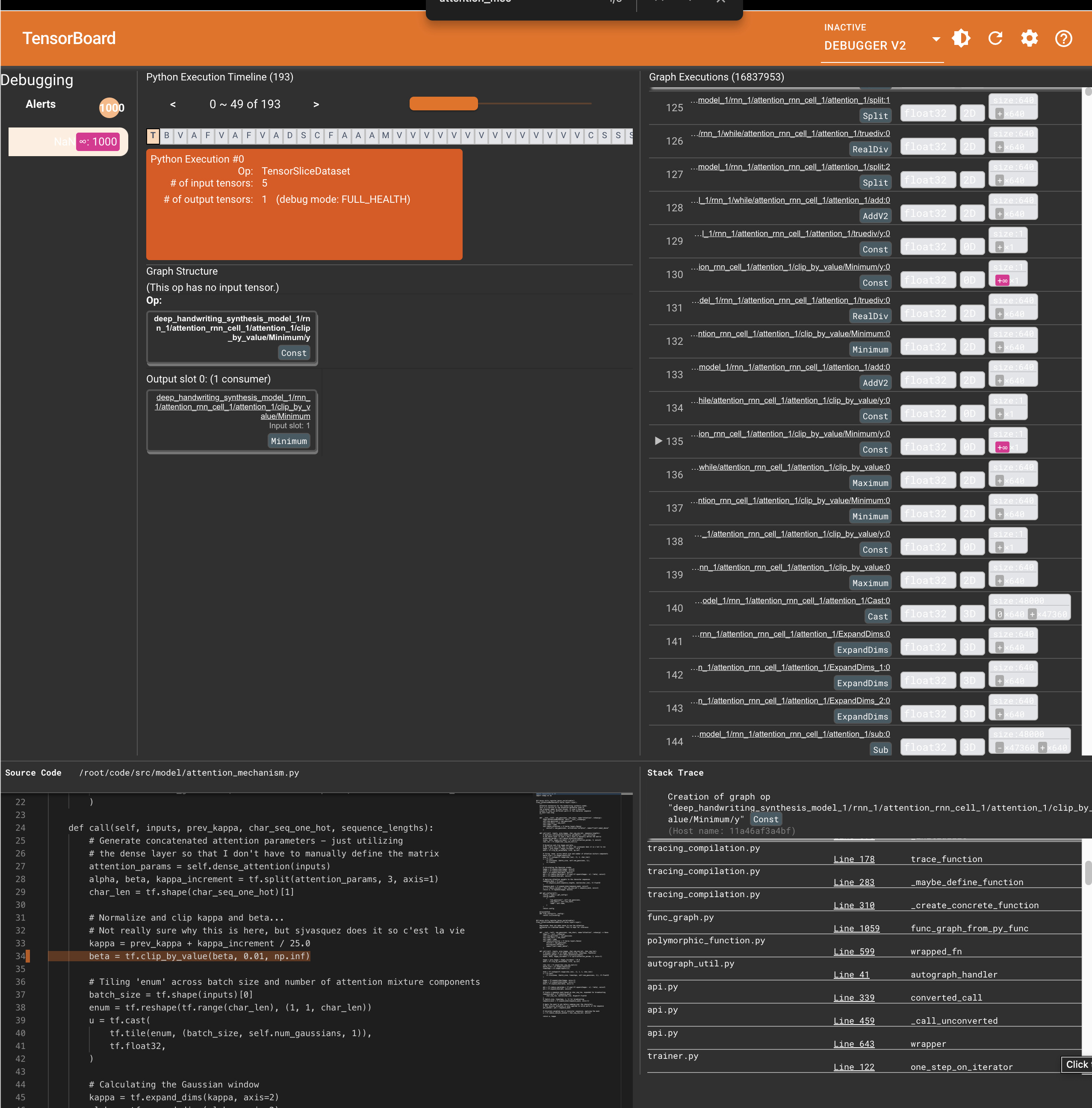
Which was even more annoying because of this: https://github.com/tensorflow/tensorflow/issues/59215 issue.
Problem #2 - OOM Galore
Uh oh, looks like the vast.ai instance I utilized didn’t have enough memory. Here is an example of one of the errors I ran into:
Out of memory error here
Out of memory while trying to allocate 22271409880 bytes.
BufferAssignment OOM Debugging.
BufferAssignment stats:
             parameter allocation:   29.54MiB
              constant allocation:         4B
        maybe_live_out allocation:   27.74MiB
     preallocated temp allocation:   20.74GiB
                 total allocation:   20.77GiB
Peak buffers:
        Buffer 1:
                Size: 3.40GiB
                Operator: op_type="EmptyTensorList" op_name="gradient_tape/deep_handwriting_synthesis_model_1/rnn_1/while/deep_handwriting_synthesis_model_1/rnn_1/while/attention_rnn_cell_1/lstm_peephole_cell_2_1/MatMul/ReadVariableOp_0/accumulator" source_file="/root/code/venv/lib/python3.11/site-packages/tensorflow/python/framework/ops.py" source_line=1177
                XLA Label: fusion
                Shape: f32[1200,476,1600]
                ==========================

        Buffer 2:
                Size: 3.40GiB
                Operator: op_type="EmptyTensorList" op_name="gradient_tape/deep_handwriting_synthesis_model_1/rnn_1/while/deep_handwriting_synthesis_model_1/rnn_1/while/attention_rnn_cell_1/lstm_peephole_cell_2_1/MatMul/ReadVariableOp_0/accumulator" source_file="/root/code/venv/lib/python3.11/site-packages/tensorflow/python/framework/ops.py" source_line=1177
                XLA Label: fusion
                Shape: f32[1200,476,1600]
                ==========================

        Buffer 3:
                Size: 2.86GiB
                Operator: op_type="EmptyTensorList" op_name="gradient_tape/deep_handwriting_synthesis_model_1/rnn_1/while/deep_handwriting_synthesis_model_1/rnn_1/while/attention_rnn_cell_1/lstm_peephole_cell_2_1/MatMul_1/ReadVariableOp_0/accumulator" source_file="/root/code/venv/lib/python3.11/site-packages/tensorflow/python/framework/ops.py" source_line=1177
                XLA Label: fusion
                Shape: f32[1200,400,1600]
                ==========================

        Buffer 4:
                Size: 2.86GiB
                Operator: op_type="EmptyTensorList" op_name="gradient_tape/deep_handwriting_synthesis_model_1/rnn_1/while/deep_handwriting_synthesis_model_1/rnn_1/while/attention_rnn_cell_1/lstm_peephole_cell_2_1/MatMul_1/ReadVariableOp_0/accumulator" source_file="/root/code/venv/lib/python3.11/site-packages/tensorflow/python/framework/ops.py" source_line=1177
                XLA Label: fusion
                Shape: f32[1200,400,1600]
                ==========================

        Buffer 5:
                Size: 2.86GiB
                Operator: op_type="EmptyTensorList" op_name="gradient_tape/deep_handwriting_synthesis_model_1/rnn_1/while/deep_handwriting_synthesis_model_1/rnn_1/while/attention_rnn_cell_1/lstm_peephole_cell_2_1/MatMul_1/ReadVariableOp_0/accumulator" source_file="/root/code/venv/lib/python3.11/site-packages/tensorflow/python/framework/ops.py" source_line=1177
                XLA Label: fusion
                Shape: f32[1200,400,1600]
                ==========================

        Buffer 6:
                Size: 556.64MiB
                Operator: op_type="EmptyTensorList" op_name="gradient_tape/deep_handwriting_synthesis_model_1/rnn_1/while/deep_handwriting_synthesis_model_1/rnn_1/while/attention_rnn_cell_1/lstm_peephole_cell_1/MatMul/ReadVariableOp_0/accumulator" source_file="/root/code/venv/lib/python3.11/site-packages/tensorflow/python/framework/ops.py" source_line=1177
                XLA Label: fusion
                Shape: f32[1200,76,1600]
                ==========================

        Buffer 7:
                Size: 219.73MiB
                Operator: op_type="While" op_name="deep_handwriting_synthesis_model_1/rnn_1/while" source_file="/root/code/venv/lib/python3.11/site-packages/tensorflow/python/framework/ops.py" source_line=1177
                XLA Label: fusion
                Shape: f32[1200,64,10,75]
                ==========================

        Buffer 8:
                Size: 219.73MiB
                Operator: op_type="While" op_name="deep_handwriting_synthesis_model_1/rnn_1/while" source_file="/root/code/venv/lib/python3.11/site-packages/tensorflow/python/framework/ops.py" source_line=1177
                XLA Label: fusion
                Shape: f32[1200,64,10,75]
                ==========================

        Buffer 9:
                Size: 219.73MiB
                Operator: op_type="While" op_name="deep_handwriting_synthesis_model_1/rnn_1/while" source_file="/root/code/venv/lib/python3.11/site-packages/tensorflow/python/framework/ops.py" source_line=1177
                XLA Label: fusion
                Shape: f32[1200,64,10,75]
                ==========================

        Buffer 10:
                Size: 139.45MiB
                Operator: op_type="While" op_name="deep_handwriting_synthesis_model_1/rnn_1/while" source_file="/root/code/venv/lib/python3.11/site-packages/tensorflow/python/framework/ops.py" source_line=1177
                XLA Label: fusion
                Shape: f32[1200,64,476]
                ==========================

        Buffer 11:
                Size: 139.45MiB
                Operator: op_type="While" op_name="deep_handwriting_synthesis_model_1/rnn_1/while" source_file="/root/code/venv/lib/python3.11/site-packages/tensorflow/python/framework/ops.py" source_line=1177
                XLA Label: fusion
                Shape: f32[1200,64,476]
                ==========================

        Buffer 12:
                Size: 139.45MiB
                Operator: op_type="While" op_name="deep_handwriting_synthesis_model_1/rnn_1/while" source_file="/root/code/venv/lib/python3.11/site-packages/tensorflow/python/framework/ops.py" source_line=1177
                XLA Label: fusion
                Shape: f32[1200,64,476]
                ==========================

        Buffer 13:
                Size: 117.19MiB
                Operator: op_type="While" op_name="deep_handwriting_synthesis_model_1/rnn_1/while" source_file="/root/code/venv/lib/python3.11/site-packages/tensorflow/python/framework/ops.py" source_line=1177
                XLA Label: fusion
                Shape: f32[1200,64,400]
                ==========================

        Buffer 14:
                Size: 117.19MiB
                Operator: op_type="While" op_name="deep_handwriting_synthesis_model_1/rnn_1/while" source_file="/root/code/venv/lib/python3.11/site-packages/tensorflow/python/framework/ops.py" source_line=1177
                XLA Label: fusion
                Shape: f32[1200,64,400]
                ==========================

        Buffer 15:
                Size: 117.19MiB
                Operator: op_type="While" op_name="deep_handwriting_synthesis_model_1/rnn_1/while" source_file="/root/code/venv/lib/python3.11/site-packages/tensorflow/python/framework/ops.py" source_line=1177
                XLA Label: fusion
                Shape: f32[1200,64,400]
                ==========================


         [[]]
Sanity Check - Validating Model Dimensions (with AI… so somewhat)
So where does AI using AI come in? I wanted to validate that the shapes of my training parameters all looked good. Again, I print out the shapes on the very first epoch to get some more details and do a quick dimensionality alignment check. I then fed that into ChatGPT along with the paper and asked it to double check all my params. Here was it’s output:
Model Summary
Model Summary
Model Name: deep_handwriting_synthesis_model
Total Parameters: 7,272,063 (27.74 MB)
Trainable Parameters: 3,636,031 (13.87 MB)
Non-Trainable Parameters: 0 (0.00 B)
Optimizer Parameters: 3,636,032 (13.87 MB)Layer-wise Breakdown
1. LSTM Peephole Cells
You have three LSTM peephole cells:
lstm_peephole_celllstm_peephole_cell_1lstm_peephole_cell_2Parameters and Shapes
For each LSTM peephole cell:
- Kernel Shape:
(input_dim, 4 * units)- Recurrent Kernel Shape:
(units, 4 * units)- Peephole Weights Shape:
(units, 3)- Bias Shape:
(4 * units,)Shapes:
First LSTM Peephole Cell (lstm_peephole_cell):
- Input Dimension: 76
- Units: 400
- Kernel Shape:
(76, 1600)(76, 4 * 400)- Recurrent Kernel Shape:
(400, 1600)(400, 4 * 400)- Peephole Weights Shape:
(400, 3)(400 units, 3 gates)- Bias Shape:
(1600,)(4 * 400,)Second and Third LSTM Peephole Cells (lstm_peephole_cell_1 and lstm_peephole_cell_2):
- Input Dimension: 476
This includes concatenated inputs from previous layers and attention outputs.- Units: 400
- Kernel Shape:
(476, 1600)(476, 4 * 400)- Recurrent Kernel Shape:
(400, 1600)(400, 4 * 400)- Peephole Weights Shape:
(400, 3)(400 units, 3 gates)- Bias Shape:
(1600,)(4 * 400,)Conclusion
The shapes of the LSTM peephole cells’ parameters are correct and align with standard LSTM architectures with peephole connections.
2. Attention Mechanism
- Layer:
attention(AttentionMechanism)Parameters and Shapes
- Kernel Shape:
(476, 30)- Bias Shape:
(30,)Explanation:
- Input Dimension: 476
This likely comes from concatenating the window vectorw, the current inputx_t, and the output from the first LSTM layers1_out.- Output Dimension: 30
Corresponds to parameters needed for the attention mechanism, such as the attention weights.Conclusion
The attention mechanism’s parameter shapes are appropriate.
3. Mixture Density Network (MDN) Layer
- Layer:
mdn(MixtureDensityLayer)Parameters and Shapes
- mdn_W_pi:
(400, 20)- mdn_b_pi:
(20,)- mdn_W_mu:
(400, 40)- mdn_b_mu:
(40,)- mdn_W_sigma:
(400, 40)- mdn_b_sigma:
(40,)- mdn_W_rho:
(400, 20)- mdn_b_rho:
(20,)- mdn_W_eos:
(400, 1)- mdn_b_eos:
(1,)Explanation:
- Hidden Units from Last LSTM Layer: 400
- Number of Mixture Components: 20
MDN Outputs:
- pi (mixture weights): 20 components
- mu (means): 2 coordinates per component * 20 components = 40 outputs
- sigma (standard deviations): 2 per component * 20 components = 40 outputs
- rho (correlation coefficients): 20 components
- eos (end-of-stroke probability): 1 output
Parameter Shapes:
- Weights:
mdn_W_pi:(400, 20)mdn_W_mu:(400, 40)mdn_W_sigma:(400, 40)mdn_W_rho:(400, 20)mdn_W_eos:(400, 1)- Biases:
mdn_b_pi:(20,)mdn_b_mu:(40,)mdn_b_sigma:(40,)mdn_b_rho:(20,)mdn_b_eos:(1,)Conclusion
The MDN layer’s parameter shapes correctly correspond to the required outputs for a mixture of 20 bivariate Gaussian components.
4. Total Parameters and Trainable Parameters
- Total Parameters: 7,272,063
- Trainable Parameters: 3,636,031
Observation:
- The total parameters are approximately double the trainable parameters.
- This may be due to counting both the weights and optimizer states (like moments in the Adam optimizer).
- Optimizer Parameters: 3,636,032 (slightly off by one, which could be due to rounding or reporting).
Conclusion
The parameter counts make sense, and the discrepancy is acceptable.
Your Model’s Parameters
All Parameters
All parameters listed are correctly shaped and correspond to their respective layers.
Trainable Parameters
All trainable parameters match the parameters in the model and have the correct shapes.
Answering Your Question
Yes, based on the model summary and the parameter shapes you’ve provided, everything appears to be in order. The shapes align with the expected dimensions > given your model’s architecture:
- LSTM Peephole Cells:
- Input dimensions and units are consistent.
- Kernels and recurrent kernels have correct shapes.
Peephole weights and biases are appropriately sized.
- Attention Mechanism:
The input and output dimensions match the concatenated inputs and expected output size.
- MDN Layer:
The weights and biases correspond correctly to the number of mixture components and the outputs required for the mixture density network.
- Parameter Counts:
- The total number of parameters is reasonable for a model of this complexity.
- The trainable parameters are correctly identified.
Final Thoughts
Proceed with Training: You can confidently continue running your training code.
- Monitoring: Keep an eye on training metrics such as loss, especially since you have confirmed that negative loss values are acceptable in your MDN context.
- Validation: Consider using a validation set to monitor overfitting and generalization performance.
- Performance Checks: If you encounter any unexpected behavior during training, revisit the data preprocessing steps and ensure that the inputs to your model are correctly shaped and normalized.
Additional Recommendations
- Logging: Utilize TensorBoard or similar tools to visualize training progress.
- Batch Size and Sequence Length: Ensure that your batch sizes and sequence lengths are manageable to prevent memory issues, as discussed earlier.
- Model Saving: Regularly save model checkpoints to avoid losing progress in case of interruptions.
✍️ Visualizations
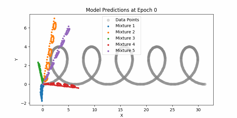
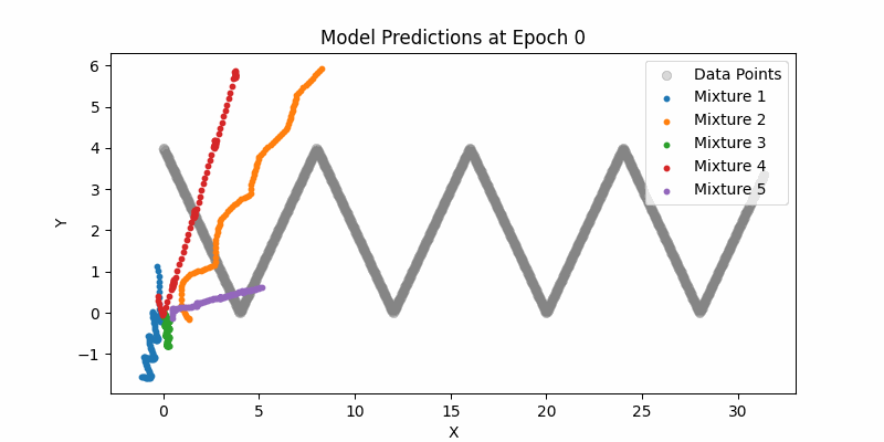
Learning with Dummy Data
Again, we used dummy data to start with to ensure our various components were learning and converging correctly.
I’m not going to burn too many pixels with these visualizations given I think they’re less interesting.
Here is our entire network and just sampling from the means (not showing the mixture densities) across the entire example datasets. One thing to note here if you can see how the LSTMs can still handle this type of larger contexts. Again, it pales in comparison to modern day transformer context, but still impressive.
Synthesis Model Sampling
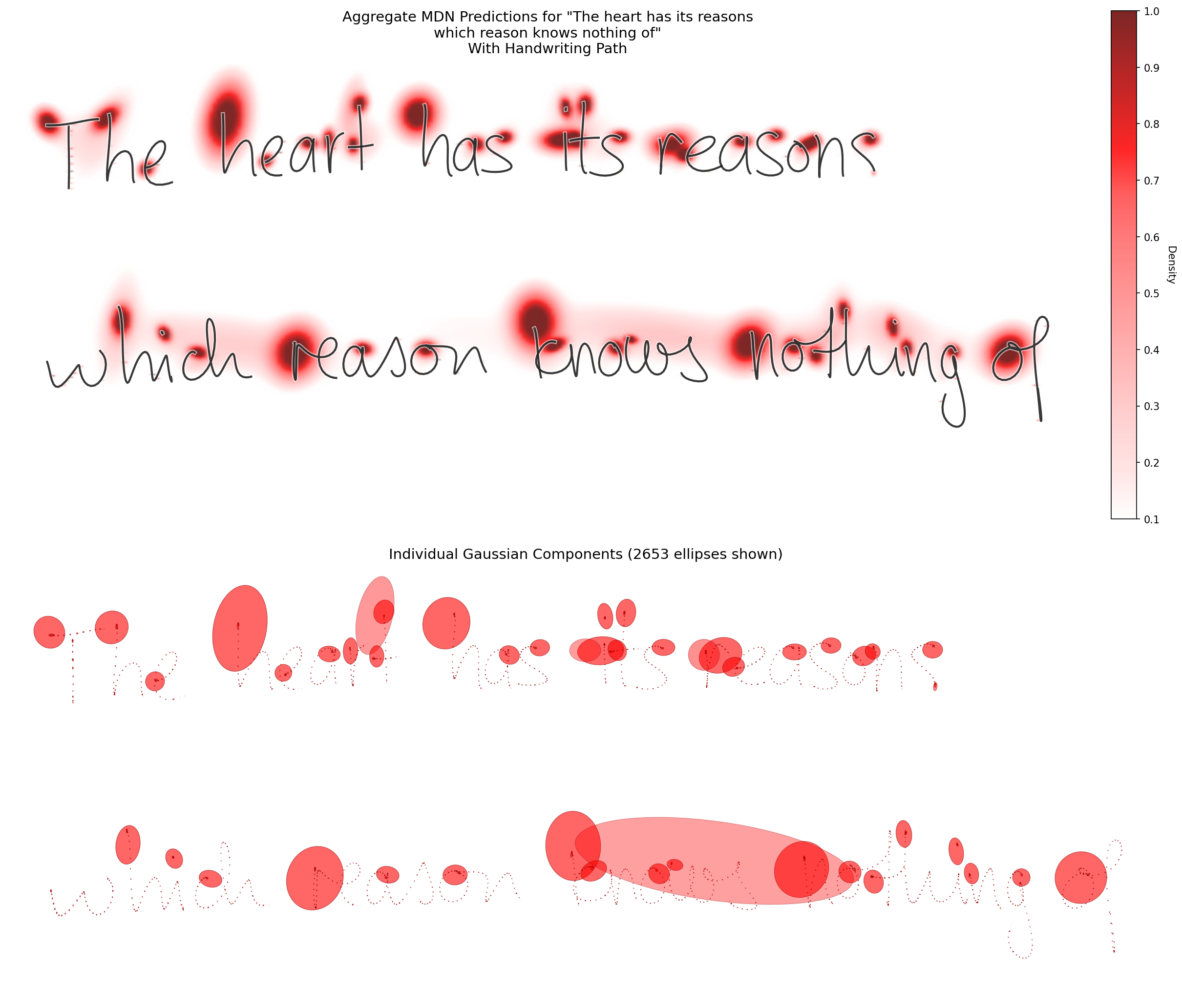
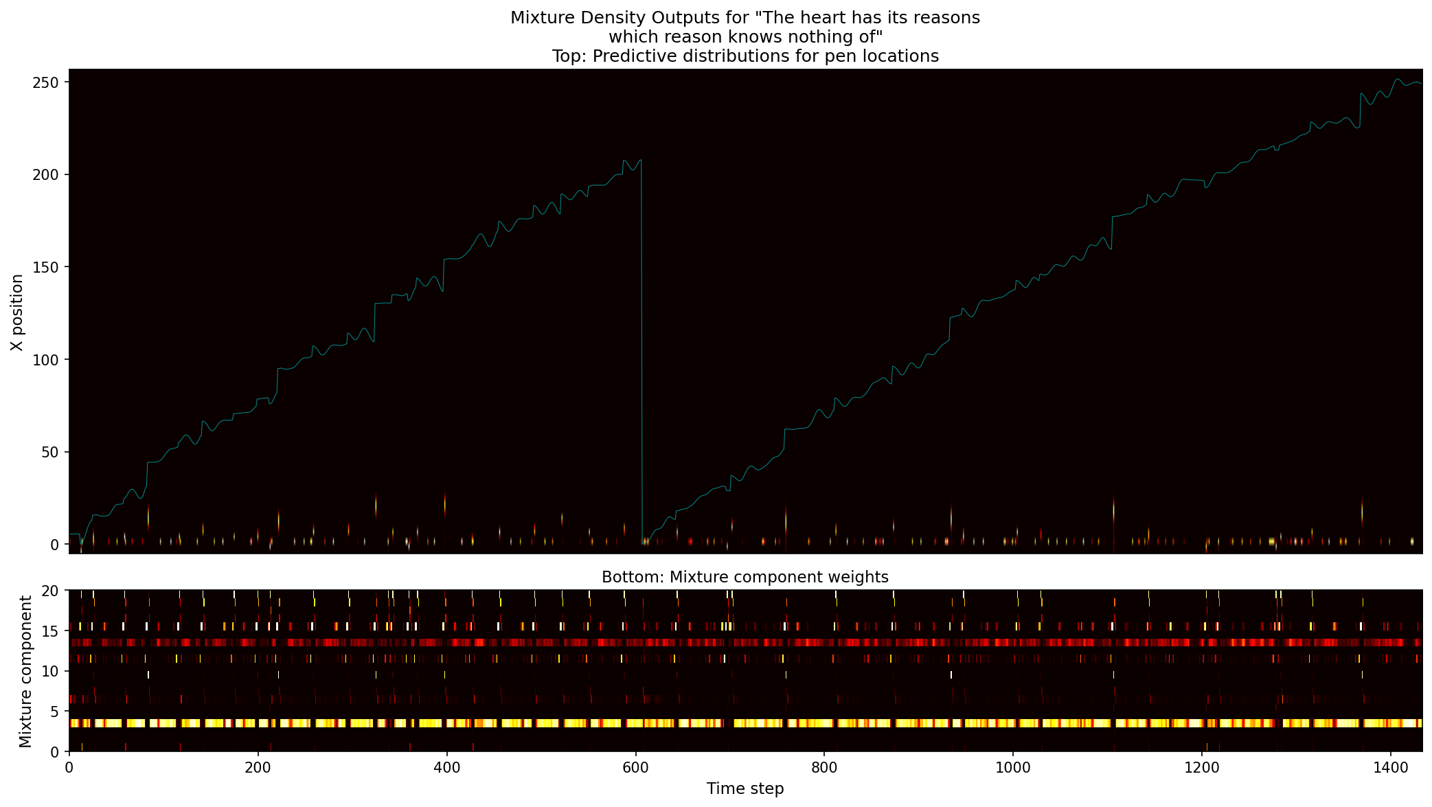
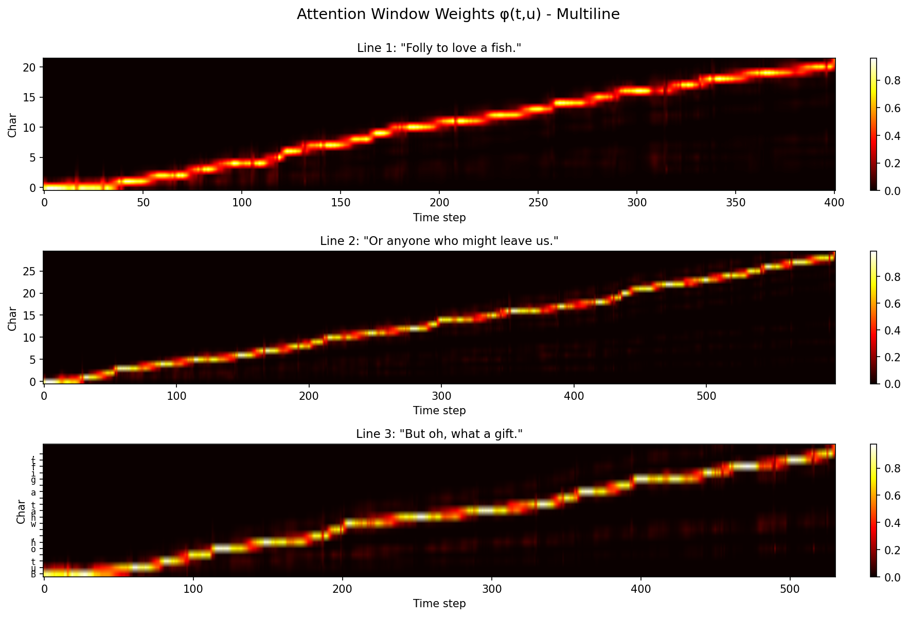
So again, given the above information, $\phi(t, u)$ represents the networks belief that it’s writing character $c_u$ at time $t$. It’s monotonically increasing (which makes sense and is enforced mathematically) and we can see its pretty stepwise increasing.
One of my favorite portions of these visualizations is the mixture components weights. You can see the various Gaussians activating for different parts of the synthesis network. For example, for end of stroke signals, we have separate Gaussians owning that portion of the model.
Most of these were generated like so:
╭─johnlarkin@Mac ~/Documents/coding/generative-handwriting-jax ‹main*›
╰─➤  uv run python generative_handwriting/generate/generate_handwriting_cpu.py \
    --checkpoint "checkpoints_saved/synthesis/loss_-2.59/checkpoint_216_cpu.pkl" \
    --text "It has to be symphonic" \
    --bias "0.75" \
    --temperature "0.75" \
    --fps "60" \
    --formats "all" \
    --seed "42"
Another note is… my termination condition logic probably could be improved. Remember, we’re doing one-hot encoding which includes the null terminator. So the null term should be at len(line_text). Attention spans the full sequence. Specifically, $\phi$ has shape [batch, char_seq_length] so we can get our single sample (i.e. batch of 0), and then look at the char sequence length to basically see where our attention is at. In code speak, here’s what I’m doing:
        # char_seq includes null terminator at index len(line_text)
        if phi is not None and t >= len(line_text) * 2:
            char_idx = int(jnp.argmax(phi[0]))
            sampled_eos = stroke[2] > 0.5

            # we can stop when:
            # 1. attention has reached the null terminator (char_idx == len(line_text)) AND we sampled EOS
            # 2. attention weight on null terminator is dominant (> 0.5)
            # 3. we're well past the text and sampled EOS multiple times
            null_attention = float(phi[0][len(line_text)]) if len(phi[0]) > len(line_text) else 0.0

            if char_idx == len(line_text) and sampled_eos:
                # this hits most
                break
            elif null_attention > 0.5:
                # attention strongly focused on null terminator
                break
            elif char_idx >= len(line_text) and t > len(line_text) * 10:
                # failsafe: past text and generated way too much
                break
Finally, on the visualization front, I’m generating everything with bias 0.75 and temperature 0.75. I’m not going to discuss those, but the original paper goes into more detail.
Heart has its reasons
The heart has its reasons which reason knows nothing of
, Pensées
One thing to note is that we are still constrained by line length. For example, if we try to specify this as a single line, we start to lose our attention and the context starts to fail. Part of this is that if we exceed the line length that we trained on (in terms of stroke sequences or input text length), then we start to flail.
So note the discrepancy between these two when we introduce a line break:
vs
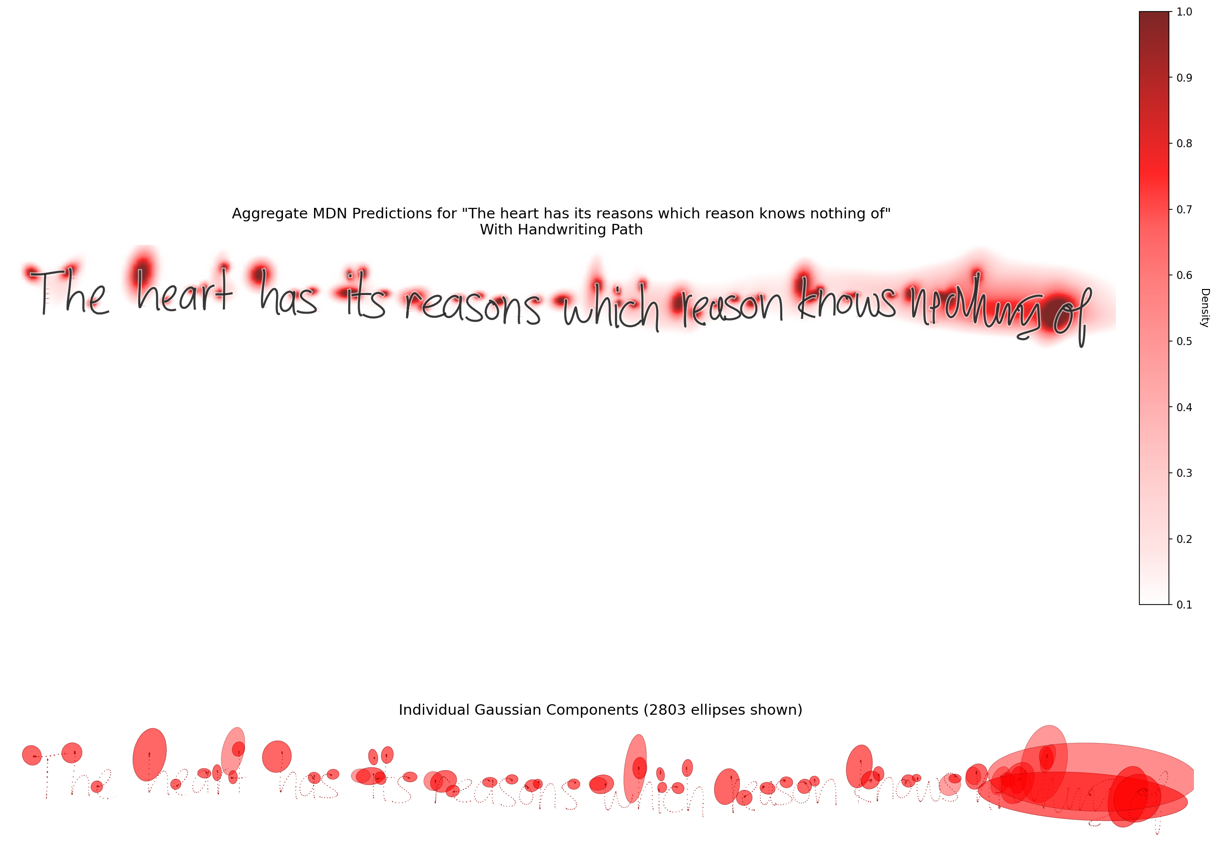
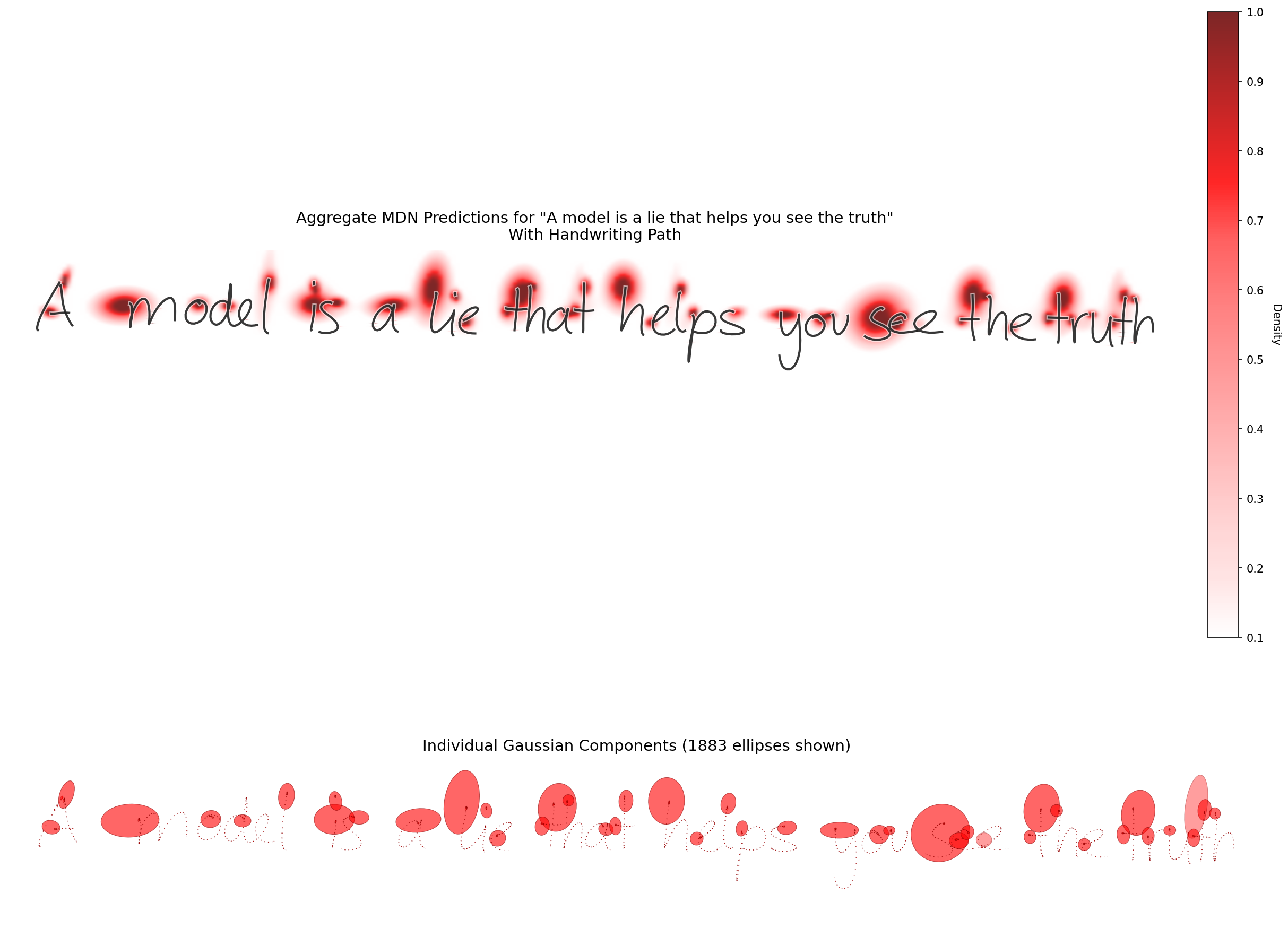
You can see how the model is less trained given the higher deviations towards the end of the line. Note, these MDN heatmap graphs on the bottom are created by showing the three highest weighted $\pi$ components per timestamp and then aggregating them across all timestamps.
Furthermore, the eos signals generally have the highest uncertainty and most spread out sigmas which makes sense given it’s the highest variable point.
Loved and lost
Better to have loved and lost than never to have loved at all
, In Memoriam A. H. H.


It has to be symphonic
It has to be symphonic
, Takeaway (The Potash Twins ft. Andrew Zimmern)

Is a model a lie?
A model is a lie that helps you see the truth
, requoted by Siddhartha Mukherjee in "The Emperor of All Maladies"


Fish folly
Hadn’t ever heard of this one but it’s my best friend’s favorite quote.
Folly to love a fish. Or anyone who might leave us. But oh, what a gift.
, I Think on Thee, Dear Friend

Conclusion
This - again - was a bit of a bear of a project. It was maybe not my best use of time, but it was a labor of love.
I don’t think I’ll embark on a project of this nature in awhile (sadly). However, I hoped the reader has enjoyed. And feel free to pull the code and dive in yourself.
When re-reading my old draft blog post, I liked the way I ended things. So here it is:
Finally, I want to leave with a quote from our academic advisor Matt Zucker. When I asked him when we know that our model is good enough, he responded with the following.
“Learning never stops.”