Table of Contents
- Table of Contents
- Motivation
- Introduction
- Goal
- Problem
- Approach
- Part 1 - Fake Data 🧑💻
- Part 2 - Theory of Hierarchical Agglomerative Clustering 👨🏫
- Part 3 - Algorithmic Approach 👾
- Part 4 - Ground Up Implementation 👷♂️
- Part 5 - Polished Implementation 💅
- Takeways - how did we do?!
Motivation
Curious how you can make such fun clustering graphs like this? Read on! Or skip to here look at the results: Takeways - how did we do?!.
Introduction
Recently, I decided to throw my hat into the interviewing arena. And with that, I got burned pretty bad for this role that I was a bit fixated with.
I have not interviewed much, and as a result, I prepped decently hard for this job interview process. While I did make it to the final day, and did well on the design and coding challenges, ultimately the company decided to pass on me given they felt they had “given me too many prompts”. I am assuming that was related to my relatively slow start in the first coding interview, and perhaps some of the open endedness of the system design question. It’s fair feedback and it’s a fair point. I don’t know if I totally agree with it, but in reality, it doesn’t matter what I believe, because it’s what they decided.

Regardless, it hurt, but I have learned from the process and will be more aware of that in the future. And hopefully I’ll be a stronger interviewee as well.
That’s only the most recent encounter I’ve had, but I’ve had a bit of a bad spell of things related to work. It’s been a rather frustrating time.
The events above are all related to the purpose of this blog post which is to take a breather, expand on a fun technical problem I saw, and clean up some code that I wanted to improve. There’s also been a boom in AI/ML related engineering, and given the links above, this problem connects those.
Abstract Thoughts
Before jumping into the problem, I want to explain a bit more about the title and the image I picked for the thumbnail of this blog post. It’s two fold:
- It feels like a constant battle to correctly answer interview questions and nail system design questions
- It is the constant question of:
Are you not entertained?
I’ll be the first to say it, I hate the interview process. I have given now hundreds of interviers to experienced candidates across big tech to juniors in college looking for their internships. It’s inheritely a terrible solution to a hard problem.
Here’s what I somewhat think comes across:
- Have you seen this interview question before?
- Can you recall time complexity analysis from college?
- Do you understand underlying data structures?
- Do you at least somewhat know how to program?
- Generally, how do you decompose problems?
What I don’t think comes across:
- Will you care about your job?
- Will you be a good teammate?
- Are you going to work hard?
To me, in terms of who I want to work with, these later points (that traditional software engineering totally misses) are just as, if not more, important than the first couple of points.
Anyway, rant over. Moving onto the fun technical stuff.
Goal
Explore a fun problem, generate a cool dendogram, and learn something new.
Problem
Here’s the gist of the problem:
Construct a rudimentary Entity Resolution (ER) pipeline. It should resolve retailer entities found in the dataset. Identical retailer entities should be linked together through Hierarchical Agglomerative Clustering (HAC).
Build a pipeline containing these steps:
- Preprocess the data
- Generate a ground truth for the dataset a. Use retailer_nm to programatically generate the ground truth b. Save to
ground_truth_labelImplement HAC from scratch
a. Use
retailer_nm_modifiedin the leastb. Linking, scoring, thresholds, are left up to you.
c. Dont use third party libraries. No
scikit-learnd. You are allowed to ues 3rd party libraries for calculating score.
Measure accuracy of solution.
a. Generate a confusion matrix to calculate precision and recall for each predicted “class”
b. Use
ground_truth_label- Persist data to pipeline_output.csv. Should contain: a. cluster_id b. ground_truth_label c. precision_for_cluster_id d. recall_for_cluster_id
$ cat pipeline_output.csv

cluster_id,ground_truth_label,precision_for_cluster_id,recall_for_cluster_id,store_record_id,retailer_id,retailer_nm,store_id,store_address_1,store_address_2,store_city,store_state,store_zip_code,store_county,vpid,retailer_nm_modified
I’m going to further simplify the problem a little bit more and just use the retailer_nm_modified.
Approach
We’re going to break down our approach into a couple of parts. Firstly, we’ll generate some fake data. Secondl, we’ll cover the theory. Thirdly, we’ll cover my thoughts from an algorithmic approach. Then, we’ll cover a custom ground up implementation, and finally, we’ll cover a solution using external packages.
Part 1 - Fake Data 🧑💻
I’m going to further simplify the problem by excluding some of the location data.
The actual problem that I saw had store_address, zip, city, etc. My thought was we could use some geodist library or some type of logic about two stores probably won’t be in the zip code (just so they’re not cannabalizing each other). However, just to protect my own time, given I’m blogging amidst the million of other things I need to do, we’ll focus on names.
So before, we even get to the algorithm, let’s generate some fake data.
Great, check out the script that did that here, but voila:
╭─johnlarkin@Larkin-Air hierarchical-agglomerative-clustering ‹main›
╰─➤  head data.csv
store_record_id,retailer_id,retailer_nm,store_id,store_address_1,store_address_2,store_city,store_state,store_zip_code,store_county,vpid,retailer_nm_modified
1,533,Target,28,mcmheyxuzfovcql,autqtndfoyyecbj,tcdudtzhgx,IL,44501,County134,24973,Targethz
2,315,Trader Joes,15,ivfptxahtmubhmt,khhsyjynsibbqgk,gppmvugarh,FL,51787,County118,35522,Trader Joes95
3,419,Walgreens,52,jthinnvoqqcnipl,forpgfpudtzyigo,myrifsmupn,TX,30360,County75,55924,qqWalgreens
4,660,Walmart,94,zmnrqzbqgfnlimd,mywwxeacltlzfyy,cshuzhvsxk,TX,81614,County41,94793,W a lmxar tx
5,848,Walmart,73,xhqrqrxmfuttvdz,tjvjgxxbhjkqxtt,lawdheatds,NY,85199,County9,42378,Walmarten
6,912,Best Buy,88,sdhpkjqdppemjlt,yproqhwpvatfnun,xiviehoifx,CA,67606,County124,40660,Best Buyfdf
7,752,Whole Foods,13,srlimmrwrgoizok,hardglbudsvaeww,cxygpjwlrb,NY,40502,County101,34246,Whole Foodsyjjq
8,532,Best Buy,96,ovbtnnrksidiihv,kcnguzspqxhwufz,xtaiwjiqya,FL,54283,County70,65235,Best Buytk
9,934,Home Depot,66,krnmvrmbybauurn,sjtzzslqoutgyhj,vawjgxzacw,OH,13184,County44,24976,Ho mxe De p o t
You can see that the data is largely garbled, but I did put some focus on just scrambling the retailer_nm_modified column, given that’s going to be where I focus (for this example). That should be good enough for now, if we need to tweak it in the future, then we can change our data gen script.
But how fake should that fake data be?
You can skip to the end, but I actually have two types of data generation, easy and hard. This was some type of check (besides the confusion matrix) that we’re clustering the easy data well, and the hard data less well.
It’s basically a toggle into the degree of simulated dirty data that we are creating. Basically, it comes down to this:
# Input
SHOULD_GENERATE_EASY = False


if SHOULD_GENERATE_EASY:
    NUMBER_OF_RECORDS = 100
    DEST_FILE = "data_easy.csv"
else:
    NUMBER_OF_RECORDS = 400
    DEST_FILE = "data_complex.csv"
and then for our generation of retailer_nm_modified field:
def modify_retailer_name(name):
    """Slightly modify the retailer name to simulate dirty data."""
    operations = [
        lambda s: s.replace(" ", ""),  # Remove spaces
        lambda s: s.lower(),  # Convert to lowercase
        lambda s: s.upper(),  # Convert to uppercase
        lambda s: " ".join(s.split()[: len(s.split()) // 2]),  # Keep first part
        lambda s: "".join(random.choice([c.upper(), c.lower()]) for c in s),  # Mixed capitalization
        lambda s: s + str(random.randint(10, 99)),  # Add numbers at the end
    ]
    if not SHOULD_GENERATE_EASY:
        operations.extend(
            [
                lambda s: s
                + random.choice([" Inc", " LLC", " Corp", " Co", " Ltd", " Corp."]),  # Add suffix
                lambda s: "".join(
                    c + random.choice(["-", "", " "]) for c in s
                ),  # Extra or missing characters
                lambda s: s + random_string(random.randint(1, 4)),  # Add random letters at the end
                lambda s: typo_generator(s),  # Introduce a typographical error
                lambda s: abbreviation(s),  # Use abbreviation
            ]
        )
    # Apply a random modification operation to the name
    modified_name = random.choice(operations)(name)
    return modified_name
Part 2 - Theory of Hierarchical Agglomerative Clustering 👨🏫
Ok so everyone’s favorite part - let’s get into the theory.
What is Hierarchical Clustering?
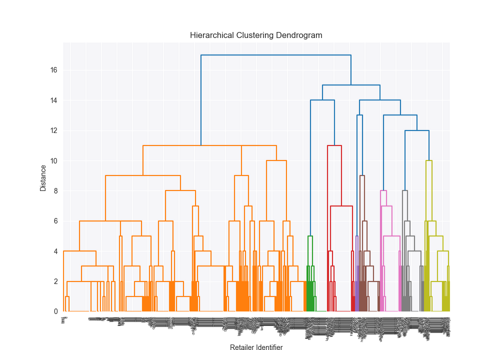
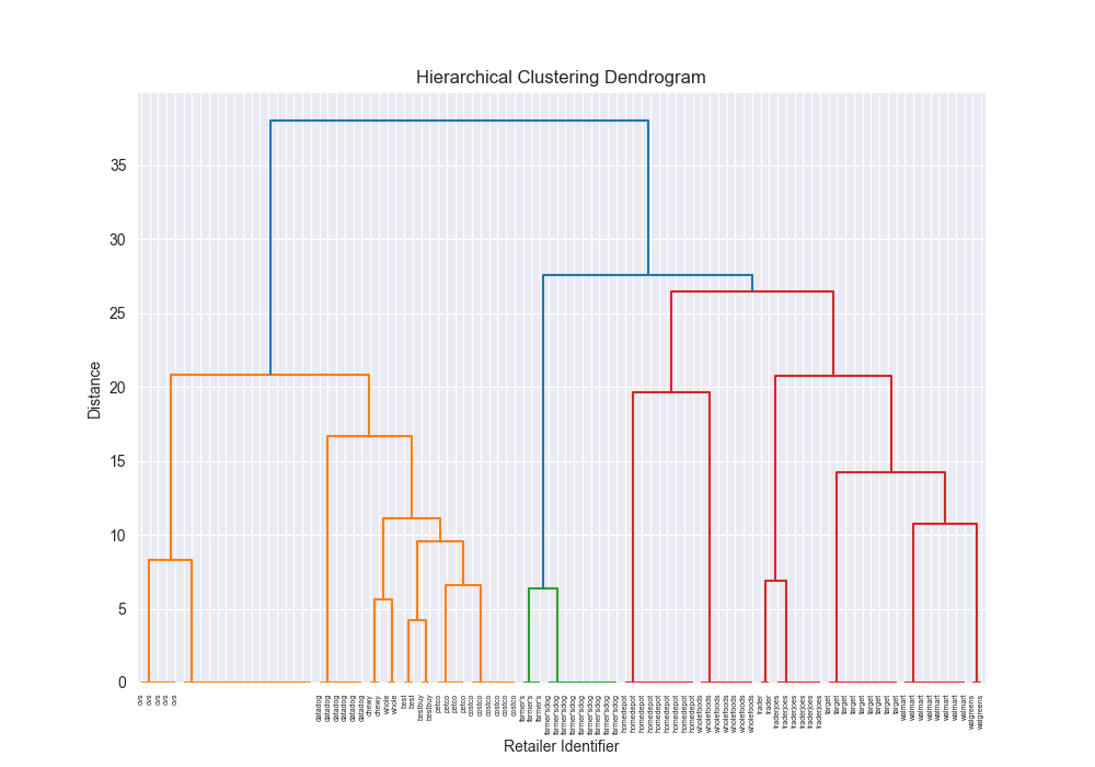
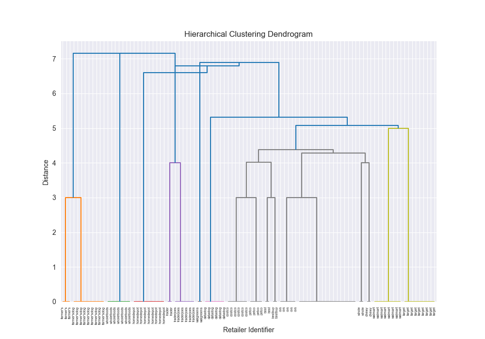
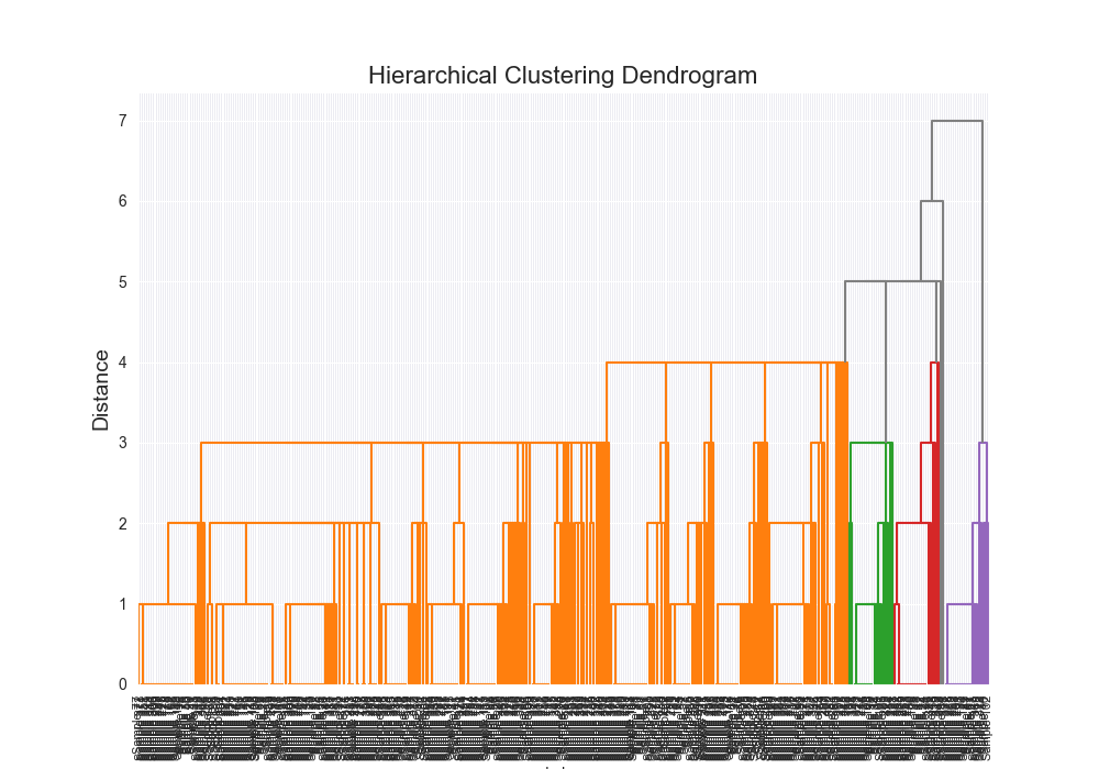
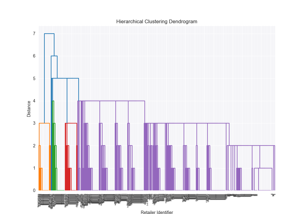
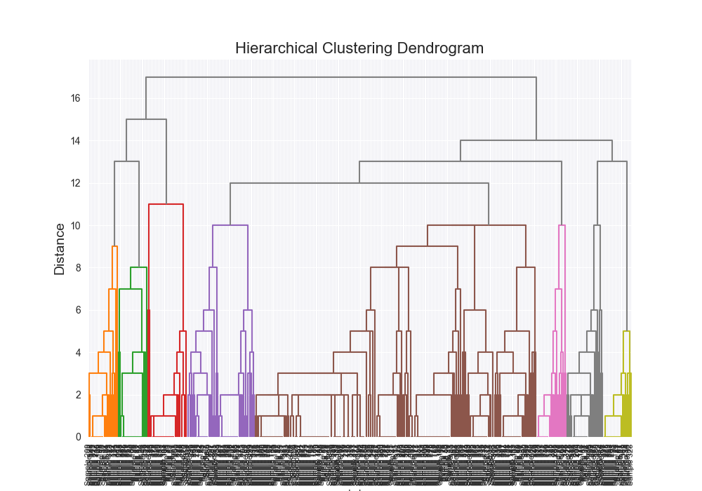
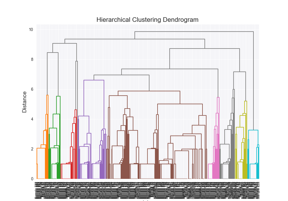
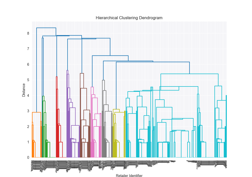
Clustering is the process of creating groups based on some characteristics. The final result is a set of clusters, where each cluster is distinct from one another in some meaningful way. Often, given that we’re focusing on hierarchical clustering, the output can be represented as a dendogram. We’ll produce one by the end of today’s blog post.
Some important points about hierarchical clustering1:
- No need to specify the number of clusters. The algorithm takes care of finding the clusters at the appropriate interval.
- Data can often by organized into a dendogram.
Visually, here are two examples.
What is Agglomerative Clustering?
You can probably get a good idea of context from the agglomerative portion (agglomerare meaning to “wind into a ball”, ad meaning “to,” and glomerare, “ball of yarn.”)
This approach starts with all of the data points as individuals. So the approach is:
- Each data point is its own cluster
- Each cluster is merged with the most similar cluster
- Repeat until only a single cluster remains
What is Divisive Clustering?
More or less, this is the opposite strategy as agglomerative. Here are all of the points start as a single cluster, and we break them down.
- All data points start as part of the same cluster
- Recursively split each cluster into smaller subcluster based on dis-similarity
Divisive clustering is much more of a “divide and conquer” type algorithm approach.
Visually, it looks like:
And yes, that’s the same gif just basically done in reverse.
We’re going to focus on agglomerative clustering.
What is a linkage?
A linkage is the criterion used to determine the distance between clusters.
So you can imagine that you have two clusters, and the linkage is basically going to be how we identify the similarity between clusters.
What are the various linkage approaches?
There are probably more, but from my research, these seem like the leading contenders:
- Minimum Linkage / Single Linkage
- Maximum Linkage / Complete Linkage
- Average Linkage
- Centroid Linkage
- Ward’s Criterion (for euclidean distances)
This slide is going to be a good illustration of the different approaches2:
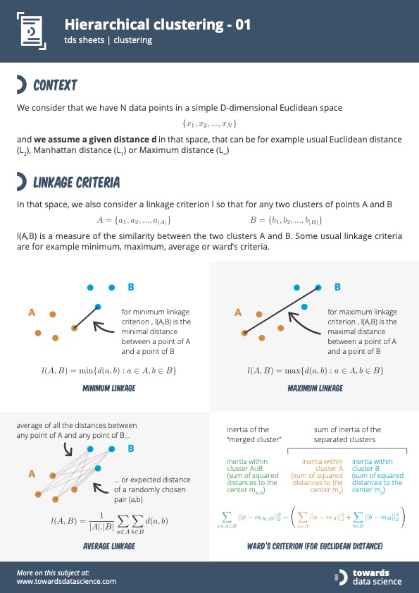
As of right now, I’ll try to support multiple types of linkage types.
What is Precision?
Precision measures the accuracy of positive predictions. It is the ratio of correctly predicted positive observations to the total predicted positive observations.
Definition
\[Precision = \frac{TP}{TP + FP}\]where
- \(TP\) = True Positives
- \(FP\) = False Positives
What is Recall?
Also called sensitivity, recall is the ability of a classifier to find all the positive samples. Ratio of correctly predicted positive observations to all of the observations in the class.
Definition:
\[Recall = \frac{TP}{TP + FN}\]where
- \(TP\) = True Positives
- \(FN\) = False Negatives
What is a Confusion Matrix?
This is relatively straight forward, and I’m utilizing sklearn.metrics ‘s confusion_matrix.
My FAVORITE visual I saw while researching the confusion matrix was here:
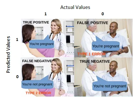
courtesy of here3.
However, for more data points, the confusion matrix basically represents these values dispersed throughout.
From their documentation,
By definition a confusion matrix C is such that C_{i, j} is equal to the number of observations known to be in group i and predicted to be in group j.
Thus in binary classification, the count of true negatives is C_{0,0}, false negatives is C_{1,0} true positives is C_{1,1}, and false positives is C_{0,1}.
What is an F1 Score?
I wanted some way to compare results with a single number for the easy vs hard data that we generated, and how well we clustered. The metric I decided to use was the weighted F1 score.
This is a way to get a single numerical value that combines aspects of recall and precision.
Part 3 - Algorithmic Approach 👾
So let’s dive into the fundamentals and a bit more of a technical breakdown about how this is going to work.
There is one main question that is abstracted by the algorithm:
- How do you identify the “distance” between clusters?
- How do you identify the new clusters center, so that you can then compare other clusters to that updated one?
How to compute distance?
Here is where we have a lot of different approaches and it kind of depends on the actual data at hand. For example, we have basically geolocation data and somewhat distorted retailer names.
There’s a lot of different approaches we could take here, but when given the actual assignment, I harkened back to my bioinformatics classes. There were two that I remembered:
- Hamming Distance
- Levenshtein Distance (although I’m positive I didn’t spell it correctly in the interview)
From the quick research, I decided on using Levenshtein distance given it’s a bit more modern and sophisticated than the hamming distance.
So the general idea is going to be, we:
- Build a matrix that shows the Levenshtein distance from one data point to the next
- Find the most similar data point based on the above distance
- Merge into a cluster
- Repeat until only a single cluster
- Generate our fun dendogram
How to identify the new clusters center?
Here is where we’re going to use the linkage type and leave the clusters as one, but just compute the distance. We’ll use Single as our linkage type, meaning we’ll be looking for the minimum.
Part 4 - Ground Up Implementation 👷♂️
This section is going to be focused on a bit more to the question I saw, where we’re doing things from the ground up so that we can better understand the actual algorithm.
This is not going to be as performant, or as fun, as part 5, so if you just want to skip to that section, be my guest.
Heart of the Implementation
You can definitely check out the code here, but I wanted to showcase the heart of the manual implementation for the Hierarchical Clustering Algorithm.
def hierarchical_clustering_from_scratch(
        self,
        should_enforce_stopping_criteria: bool = False,
    ) -> pd.DataFrame:
        """
        Performs the hierarchical clustering algorithm.

        1. Builds our distance matrix.
        2. Initiative all points as their own cluster.
        3. Finds the closest clusters.
        4. Iteratively merges the closest clusters.
        5. Updates the distance matrix.
        6. Repeat steps 3-5 until we have a single cluster.
        """

        # 1. Build distance matrix
        @timing_decorator
        def build_distance_matrix(data: pd.DataFrame) -> np.ndarray:
            """
            Builds the distance matrix for our data.

            The distance matrix is a square matrix that contains the pairwise distances
            between each point in our data.
            """

            num_rows = len(self.processed_data["retailer_nm_modified"].values)
            distance_matrix = np.zeros((num_rows, num_rows))
            for i in range(num_rows):
                for j in range(i + 1, num_rows):
                    distance = compute_distance(data.iloc[i], data.iloc[j])
                    # distance matrix is symmetrical
                    distance_matrix[i, j] = distance
                    distance_matrix[j, i] = distance
            return distance_matrix

        distance_matrix = build_distance_matrix(self.processed_data)
        n = len(self.processed_data)
        cluster_id_to_dendrogram_index = {i: i for i in range(n)}
        next_cluster_index = n
        dendrogram_data = []

        # 2. Initialize all points as their own cluster
        self.processed_data["cluster_id"] = self.processed_data.index
        index_to_cluster_id: dict[int, int] = {
            i: cluster_id for i, cluster_id in enumerate(self.processed_data["cluster_id"])
        }

        @timing_decorator
        def find_closest_clusters(
            distance_matrix: np.ndarray,
            index_to_cluster_id: dict[int, int],
        ) -> tuple[int, int, int, int]:
            """
            Finds the two closest clusters in our data.

            We'll use the distance matrix to find the two closest clusters.
            """
            min_val = np.inf
            cluster_index_a, cluster_index_b = -1, -1
            for i in range(distance_matrix.shape[0]):
                for j in range(i + 1, distance_matrix.shape[1]):  # Ensure i != j
                    # Check if i and j belong to different clusters before comparing distances
                    if (
                        distance_matrix[i, j] < min_val
                        and index_to_cluster_id[i] != index_to_cluster_id[j]
                    ):
                        min_val = distance_matrix[i, j]
                        cluster_index_a, cluster_index_b = i, j

            cluster_a_id = index_to_cluster_id[cluster_index_a]
            cluster_b_id = index_to_cluster_id[cluster_index_b]
            # Additional check to ensure cluster IDs are distinct could be added here, if necessary
            return cluster_a_id, cluster_b_id, cluster_index_a, cluster_index_b

        @timing_decorator
        def merge_closest_clusters(
            cluster_a: int,
            cluster_b: int,
            cluster_index_a: int,
            cluster_index_b: int,
        ) -> pd.DataFrame:
            """
            Merges the two closest clusters in our actual dataframe.
            We don't touch our distance matrix yet.

            We'll merge the two closest clusters and update the cluster_id column
            in our data.
            """
            nonlocal next_cluster_index

            # Update the cluster_id for all points in cluster_b
            self.processed_data.loc[
                self.processed_data["cluster_id"] == cluster_b, "cluster_id"
            ] = cluster_a
            merge_distance = distance_matrix[cluster_index_a, cluster_index_b]
            new_cluster_size = len(
                self.processed_data[self.processed_data["cluster_id"] == cluster_a]
            )
            dendrogram_data.append(
                [
                    cluster_id_to_dendrogram_index[cluster_a],
                    cluster_id_to_dendrogram_index[cluster_b],
                    merge_distance,
                    new_cluster_size,
                ]
            )

            cluster_id_to_dendrogram_index[cluster_a] = next_cluster_index
            cluster_id_to_dendrogram_index[cluster_b] = next_cluster_index

            next_cluster_index += 1  # Prepare for the next merge
            return self.processed_data

        @timing_decorator
        def update_distance_matrix(dist_matrix: np.ndarray, cluster_a: int, cluster_b: int) -> None:
            # We always merge cluster_b into cluster_a
            for idx, cluster_id in list(index_to_cluster_id.items()):
                if cluster_id == cluster_b:
                    index_to_cluster_id[idx] = cluster_a

            # Set diagonal to np.inf to ignore self-distances
            np.fill_diagonal(dist_matrix, np.inf)

            # Recompute distances for the new cluster
            # We only need to update the distances for when
            # the distance matrix is referencing cluster_a or cluster_b
            for i in range(len(dist_matrix)):
                for j in range(len(dist_matrix)):
                    # Get the cluster IDs for points i and j
                    cluster_id_i = index_to_cluster_id.get(i)
                    cluster_id_j = index_to_cluster_id.get(j)

                    # If i or j is part of the newly merged cluster, recalculate the distance
                    if cluster_id_i == cluster_a or cluster_id_j == cluster_a:
                        new_distance = calculate_new_distance(
                            cluster_a,
                            cluster_b,
                            cluster_id_j if cluster_id_i == cluster_a else cluster_id_i,
                            self.linkage_type,
                            dist_matrix,
                            index_to_cluster_id,
                        )
                        dist_matrix[i][j] = new_distance
                        dist_matrix[j][i] = new_distance
            return dist_matrix, index_to_cluster_id

        # Now we loop until we have a single cluster
        unique_retailer_count = len(self.processed_data["retailer_nm"].unique())
        while len(self.processed_data["cluster_id"].unique()) > (
            unique_retailer_count
            if (should_enforce_stopping_criteria or self.should_enforce_stopping_criteria)
            else 1
        ):
            print("Number of clusters:", len(self.processed_data["cluster_id"].unique()))
            start_time = time.time()

            # 3. Find the closest clusters
            cluster_a, cluster_b, cluster_index_a, cluster_index_b = find_closest_clusters(
                distance_matrix, index_to_cluster_id
            )
            # 4. Merge the closest clusters in our
            self.processed_data = merge_closest_clusters(
                cluster_a, cluster_b, cluster_index_a, cluster_index_b
            )
            # 5. Update the distance matrix
            distance_matrix, index_to_cluster_id = update_distance_matrix(
                distance_matrix, cluster_a, cluster_b
            )

            end_time = time.time()
            elapsed_time = end_time - start_time
            print("Elapsed time of clustering loop:", elapsed_time, "seconds")

        # Only try to show the dendrogram if we have the full merge history
        if not should_enforce_stopping_criteria and not self.should_enforce_stopping_criteria:
            sns.set_style("darkgrid")
            plt.figure(figsize=(10, 7))
            linkage_matrix = np.array(dendrogram_data)
            np.savetxt("data/output/linkage_matrix.csv", linkage_matrix, delimiter=",")
            print("Dendrogram Data:", dendrogram_data)

            n_clusters = linkage_matrix.shape[0] + 1
            labels = [f"Sample {i+1}" for i in range(n_clusters)]

            dendrogram(
                linkage_matrix,
                orientation="top",
                labels=labels,
                distance_sort="descending",
                show_leaf_counts=True,
                leaf_rotation=90.0,
                leaf_font_size=8.0,
                color_threshold=0.7 * max(linkage_matrix[:, 2]),
                above_threshold_color="grey",
            )

            plt.title("Hierarchical Clustering Dendrogram", fontsize=16)
            plt.xlabel("Index", fontsize=10)
            plt.ylabel("Distance", fontsize=14)
            plt.savefig(self.output_dendrogram_path)
            plt.show()

        return self.processed_data
Questions that Arose
Early Stopping Criterion
One thing to note is that the whole point of the Hierarchical Clustering Algorithm is that we converge to a single cluster. That’s a little bit different than what we want here, because we want to have a cluster_id per each retailer. So there’s two things we can do here: 1) stop when we have the number of clusters we know (given we have the retailer_nm and so we’ll know the number of unique clusters) 2) generate an interactive dendrogram and then try to pick various cutoff points based on the number of clusters.
As a result, in our slight variation of Hierarchical Clustering Algorithm, we’re going to implement a stopping criterion which correlates to the number of unique retailer names.
Mapping Generated ClusterIds to Ground Truth Label
So we’ll have our early stopping criterion, but then the question arises of how do we map OUR generated cluster_ids to the ground_truth_labels.
I think the best way to do this is to identify per our computed cluster the most frequent (i.e. the mode) ground_truth_label that we’ve seen and then map it accordingly.
Basically, a simple example would be like this:
>>> import pandas as pd
>>> import numpy as np
>>>
>>> data = {'ground_truth_label': [1, 1, 1, 2, 2, 3, 7],
...         'cluster_id': [7, 7, 6, 6, 6, 2, 1]}
>>> df = pd.DataFrame(data)
>>>
>>> # Group by cluster_id and ground_truth_label, and count occurrences
>>> grouped = df.groupby(['cluster_id', 'ground_truth_label']).size().reset_index(name='count')
>>>
>>> # Sort the grouped data to ensure the mode (highest count) comes first
>>> grouped_sorted = grouped.sort_values(by=['cluster_id', 'count'], ascending=[True, False])
>>>
>>> # Drop duplicates to ensure one-to-one mapping, keeping the first occurrence (the mode)
>>> unique_mapping = grouped_sorted.drop_duplicates(subset='cluster_id', keep='first')
>>>
>>> # Create the mapping dictionary
>>> mapping_dict = pd.Series(unique_mapping.ground_truth_label.values,index=unique_mapping.cluster_id).to_dict()
>>>
>>> print(mapping_dict)
{1: 7, 2: 3, 6: 2, 7: 1}
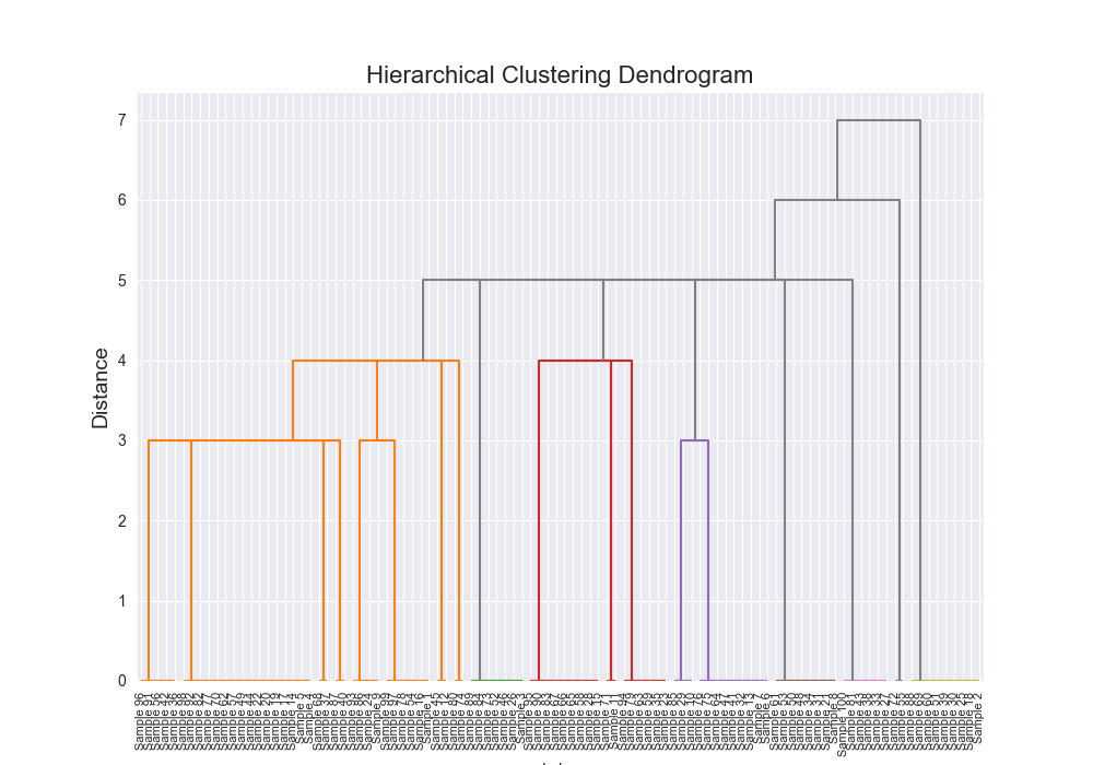
Plotting a Dendrogram
For sure the most annoying part of this whole project was trying to build out the apporpriate linkage matrix to pass to scipy’s dendrogram.
Partially the issue was indexing and partially the issue was that we’re stopping early so some of the structure about the linkage matrix (described here) was inherently incorrect.
It was annoying, but if you want to see some fun visualizations, check it out here: Dendrogram Visualization.
Part 5 - Polished Implementation 💅
So again, all of the above, and all of the code found here was largely aimed at implementing the hierarchical clustering algorithm from scratch.
This section is trying to utilize 3rd party libraries to perform that our self.
At first I thought it would be best if there was two separate scripts to do the clustering, but after writing the code, I decided that some input or feature flags at the top of the script would work just as well.
So I refactored my code to include this portion.
SHOULD_USE_THIRD_PARTY = False

# more code

    @timing_decorator
    def hierarchical_clustering(
        self,
        should_enforce_stopping_criteria: bool = False,
    ) -> pd.DataFrame:
        if SHOULD_USE_THIRD_PARTY:
            return self.hierarchical_clustering_from_third_party()
        return self.hierarchical_clustering_from_scratch(should_enforce_stopping_criteria)
The actual implementation is very simple, so I’ll include that here:
    def hierarchical_clustering_from_third_party(self) -> pd.DataFrame:
        """
        Performs the hierarchical clustering algorithm using a third-party library.
        """
        retailer_nm_modified = self.processed_data["retailer_nm_modified"].values

        # Calculate the Levenshtein distance matrix in a condensed form
        n = len(retailer_nm_modified)
        condensed_dist_matrix = np.zeros(n * (n - 1) // 2)
        k = 0
        for i in range(n):
            for j in range(i + 1, n):
                condensed_dist_matrix[k] = levenshtein_distance(
                    retailer_nm_modified[i], retailer_nm_modified[j]
                )
                k += 1

        Z = linkage(condensed_dist_matrix, self.linkage_type.value)

        desired_clusters = len(self.processed_data["retailer_nm"].unique())
        cluster_labels = fcluster(Z, desired_clusters, criterion="maxclust")
        self.processed_data["cluster_id"] = cluster_labels
Takeways - how did we do?!
Honestly? Pretty well!
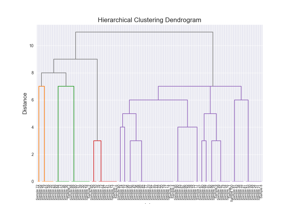
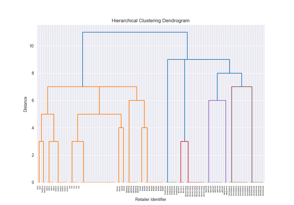
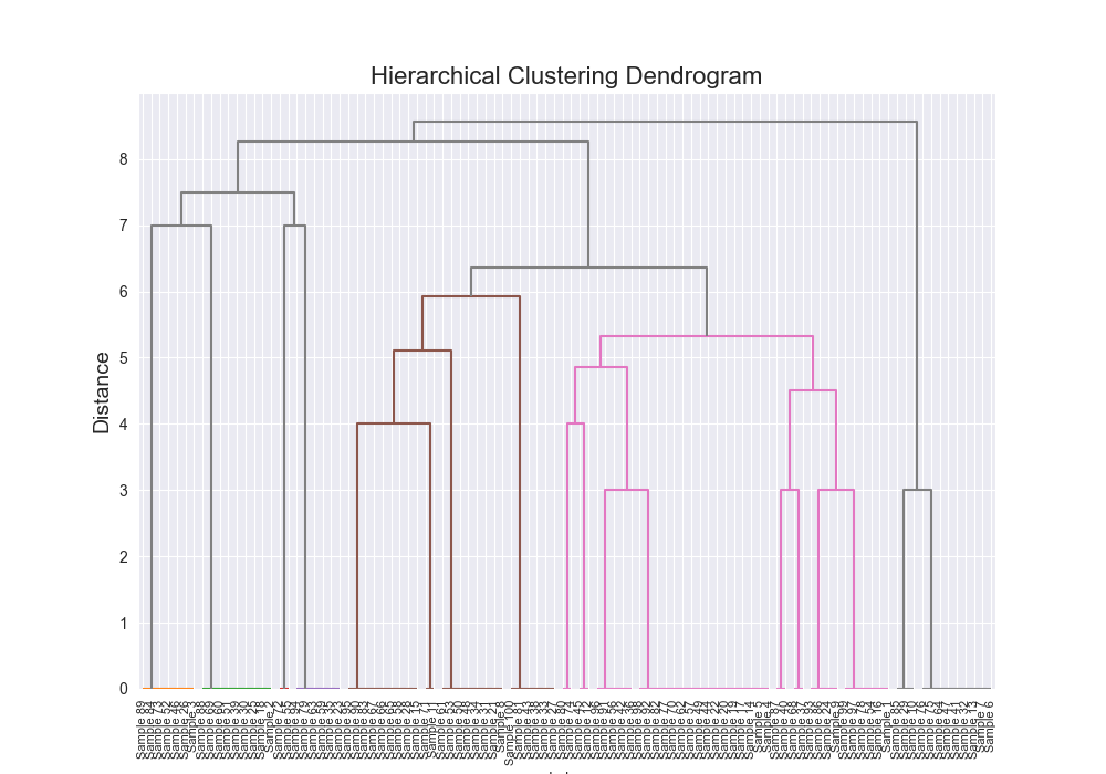
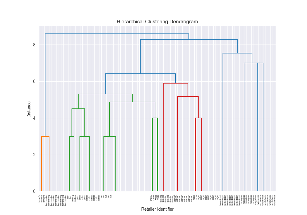
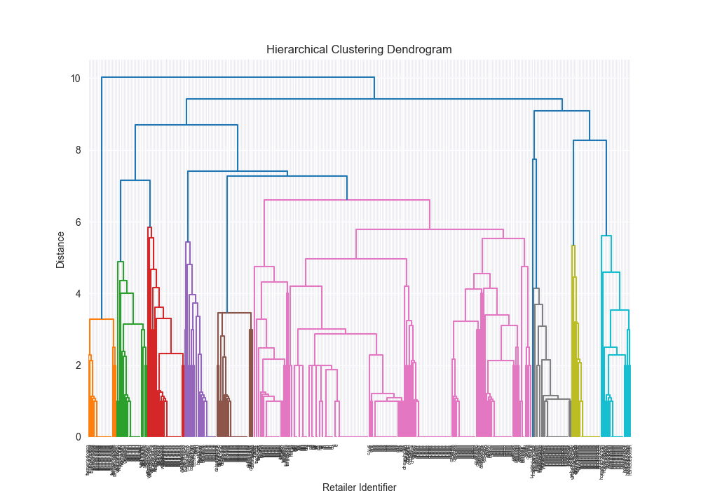
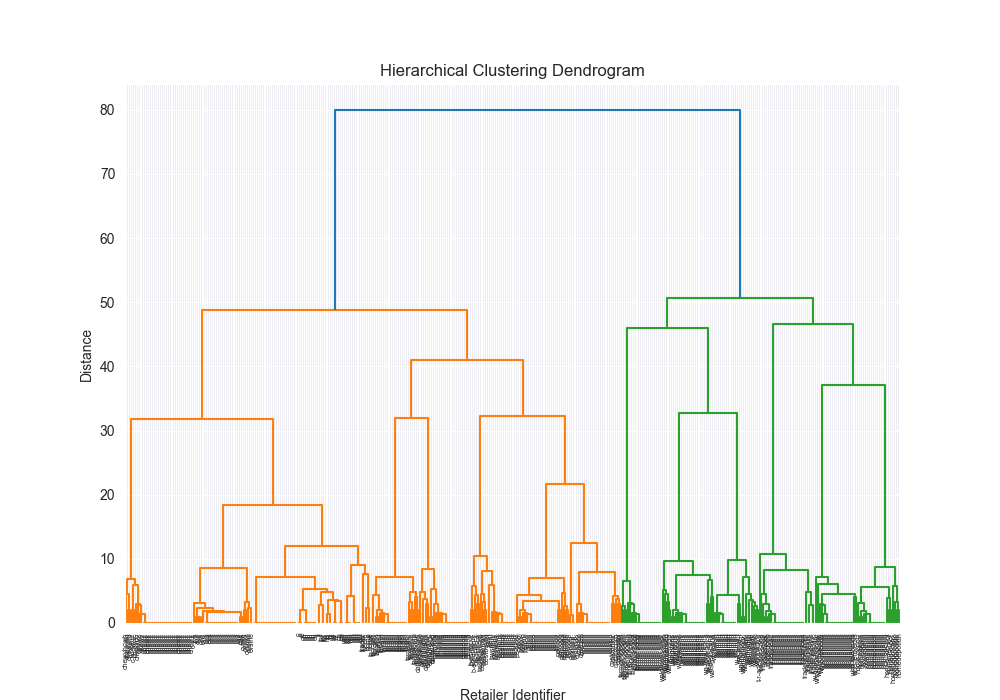
| Dataset | Distance Algorithm | Linkage Method | Implementation | F1 Score | Confusion Matrix | Dendrogram (feel free to open in new tab!) | Time for Algo Step (full clustering, seconds) |
|---|---|---|---|---|---|---|---|
| simple | levenshtein | single | scratch | 0.7934 |
|  | 44.7954 |
| simple | levenshtein | single | 3rd party | 0.7934 |
|  | 2.8021 |
| simple | levenshtein | complete | scratch | 0.8203 |
|  | 27.1838 |
| simple | levenshtein | complete | 3rd party | 0.7913 |
|  | 5.2054 |
| simple | levenshtein | average | scratch | 0.8203 |
|  | 72.2544 |
| simple | levenshtein | average | 3rd party | 0.7913 |
|  | 2.7315 |
| simple | levenshtein | ward | scratch | N/A | N/A | N/A | N/A |
| simple | levenshtein | ward | 3rd party | 0.8118 |
|  | 2.2091 |
| simple | levenshtein | centroid | scratch | N/A | N/A | N/A | N/A |
| simple | levenshtein | centroid | 3rd party | 0.8118 |
|  | 1.7993 |
| complex | levenshtein | single | scratch | 0.2283 |
|  | 87855.6781 |
| complex | levenshtein | single | 3rd party | 0.2045 |
|  | 2.0232 |
| complex | levenshtein | complete | scratch | 0.7025 |
|  | 7232.4973 |
| complex | levenshtein | complete | 3rd party | 0.6157 |
| | 2.1442 |
| complex | levenshtein | average | scratch | 0.6955 |
|  | 12005.9713 |
| complex | levenshtein | average | 3rd party | 0.6937 |
|  | 1.9224 |
| complex | levenshtein | ward | scratch | N/A | N/A | N/A | N/A |
| complex | levenshtein | ward | 3rd party | 0.8711 |
|  | 3.3757 |
| complex | levenshtein | centroid | scratch | N/A | N/A | N/A | N/A |
| complex | levenshtein | centroid | 3rd party | 0.6248 |
|  | 3.7413 |
One of the most satisfying things about this was seeing that there were some exact alignments between my implementation and the third party implementation.
There were also some discrepancies which I kind of figure is because of various optimizations and the fact that scipy’s example is probably doing some more advanced stuff under the hood, but seeing similar results across the board, made me feel pretty good about my implementation, and furthermore, my understanding that I had fully grokked how this algorithm works.
Misses 🎯
Performance
My implementation was obviously a lot slower, so that wasn’t great. Granted some of those timing metrics are skewed because I was traveling and so the timing got a bit messed up, but there were some serious compute times given the serial way we were updating our distance functioon.
Distance Function
I think Levenshtein distance is still optimal, but I wanted to also explore the Jaro-Winkler Distance, and then also explore a combination of both of them. That being said… for the sake of time I’ve already spent on this blog post, I did not get a chance to. I constrained myself to only using Levenshtein distance, but I’d be curious about trying others.
Wins 🎉
Accuracy
Pretty good F1 scores! Which was exciting to see. Our native results were pretty compartive to the 3rd party scipy solution.
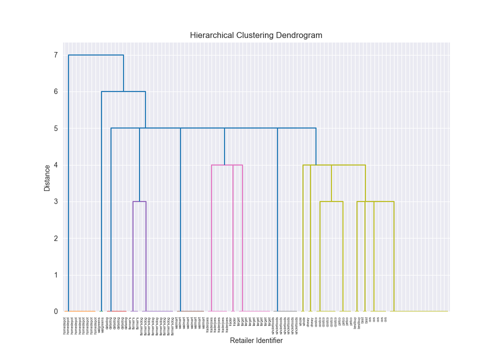
Beautiful Visualizations
See below, but I think these are pretty fun to look at and analyze.
Deeper Understanding and New Technical Skills
I learned a ton during this process and I was pretty fired up with what I built and this post. It’s definitely one of my favorites.
Next Steps 🪜
It’d be lovely if we could try different distance functions.
Dendrogram Visualization