An homage to Matt and Swarthmore.

Background

This has actually been a long time coming. I first touched this file for this blog post and dated it 2018-05-17-duals.md. Which is awhile ago. But I am finalllllly getting back to it.

I distinctively remember this topic first getting introduced in the spring of 2016 Matt Zucker in Numerical Methods. I think - if i recall correctly - that it was a one day aside basically just to show us a different vector space of our normal mathematical field (like real numbers and the such). I was blown away because basically what it offered was automatic differentiation. To me, it literally looked like Matt was doing magic up there. And he kind of was, enchanting a class like that. But it turns out that now this type of number system is used in Tensorflow and Keras and other computing platforms to expedite differentiation. It’s a really interesting different type of number system to work with.

Code

Note, if you’re just interested in code, you can skip all this and check out this repo.

Mathematical Introduction

Ok so! There’s a really good relatively quick introduction video here. Also ironically enough, that video is pretty recent. However, I’m going to put it in my own words as both a visual refresher and a refresher for myself.

We’re going to define duals as the set of numbers \(a + b \varepsilon\) where \(a\) and \(b\) are real numbers.

This epsilon is going to have one (maybe two) overarching principles to allow us to unlock this number space.

\[{\varepsilon}^2 = 0\]
\[\frac{\varepsilon}{\varepsilon} = 1\]

The premise that we’re going to assert is that this \(\varepsilon\) is going to be a number that is extremely small, and so that when it’s squared, it’s equal to zero. This is going to be a number system that pins itself on that assumption.

Now there’s a whole lot more to this in terms of number theory and abstract algebra that I’m not going to get into here. Wikipedia has a quote saying:

In abstract algebra, the algebra of dual numbers is often defined as the quotient of a polynomial ring over the real numbers \({\displaystyle (\mathbb {R} )}\) by the principal ideal generated by the square of the indeterminate

Which is a bit outside of my pay grade… I don’t know anything about quotient rings, but the polynomial ring seems to be a ring (basically a field of math) with one or more indeterminates in one ring, and coefficients in another ring. That makes sense to be given that we’re combining numbers between the real number system and our new dual number system.

You’ll also note that this is really similar to the imaginary number system. The basic difference is that in imaginary systems we have \(i^2 = -1\) whereas with dual numbers we have \({\varepsilon}^2 = 0\).

Benefits

What’s the benefit? Well we’re going to show it down below, but the real benefit is that we can evaluate a derivative at a point instantaneously and without any algebra. This is an incredibly powerful tool.

Operations

Addition

Similar to imaginary numbers, we can simply add component wise. So

\[\begin{align*} d_1 &= a_1 + b_1 \varepsilon \\ d_2 &= a_2 + b_2 \varepsilon \\ d_1 + d_2 &= (a_1 + a_2) + (b_1 + b_2) \varepsilon \end{align*}\]

Multiplication

This is where it starts to get fun.

\[\begin{align*} d_1 &= a_1 + b_1 \varepsilon \\ d_2 &= a_2 + b_2 \varepsilon \\ d_1 \cdot d_2 &= (a_1 \cdot a_2) + (a_1 \cdot b_2 + a_2 \cdot b_1)\varepsilon + (b_1 \cdot b_2) \varepsilon^2 \\ d_1 \cdot d_2 &= (a_1 \cdot a_2) + (a_1 \cdot b_2 + a_2 \cdot b_1)\varepsilon && \text{ because of } \varepsilon^2 = 0 \end{align*}\]

Subtraction

Similar to addition:

\[\begin{align*} d_1 &= a_1 + b_1 \varepsilon \\ d_2 &= a_2 + b_2 \varepsilon \\ d_1 - d_2 &= (a_1 - a_2) + (b_1 - b_2) \varepsilon \end{align*}\]

Division

So this was interesting, because I didn’t remember this from school, but Wikipedia had a good idea. It makes sense to multiply by the conjugate and you get a slightly different expression.

\[\begin{align*} d_1 &= a_1 + b_1 \varepsilon \\ d_2 &= a_2 + b_2 \varepsilon \\ \frac{d_1}{d_2} &= \frac{a_1 + b_1\varepsilon }{a_2 + b_2 \varepsilon} \\ &= \frac{(a_1 + b_1\varepsilon)(a_2 - b_2 \varepsilon)}{(a_2 + b_2 \varepsilon)(a_2 - b_2 \varepsilon)} \\ &= \frac{a_1 a_2 + (a_2 b_1 - a_1 b_2)\varepsilon - b_1 b_2 \varepsilon^2 } {a_2^2 + a_2 b_2 \varepsilon - a_2 b_2 \varepsilon - b_2^2 \varepsilon^2 } \\ &= \frac{a_1 a_2 + (a_2 b_1 - a_1 b_2)\varepsilon - \color{red}{b_1 b_2 \varepsilon^2 }} {a_2^2 + \color{red}{a_2 b_2 \varepsilon} - \color{red}{a_2 b_2 \varepsilon} - \color{red}{b_2^2 \varepsilon^2 }} \\ &= \frac{a_1 a_2 + (a_2 b_1 - a_1 b_2)\varepsilon} {a_2^2 } \\ &= \frac{a_1}{a_2} + \frac{a_2 b_1 - a_1 b_2}{a_2^2} \varepsilon \end{align*}\]

Exponents

This is another kind of interesting area where I had to think about it and actually broke out some pen and paper, before realizing the solution.

So how do we handle raising a dual number to a set power? Well… we really only have to worry about the first two terms right? If we know that \(\varepsilon^2\) is going to be zero, then we really only need to worry about the real portion and then when \(\varepsilon\) is raised to the first power. Everything else (\(\varepsilon^2\), \(\varepsilon^3\), and so forth) are just going to cancel out to zero. Beautiful. It’s really going to be the first derivative. So we can generalize:

\[\begin{align*} d^n &= (a + b \varepsilon)^n \\ &= \binom{n}{0} a^n (b\varepsilon)^0 + \binom{n}{1}a^{n-1}b\varepsilon + \binom{n}{2}a^{n-2}(b\varepsilon)^2 + \binom{n}{3}a^{n-3}(b\varepsilon)^3 + \ldots \\ &= \binom{n}{0}a^n (b\varepsilon)^0 + \binom{n}{1}a^{n-1}b\varepsilon + \color{red}{\binom{n}{2}a^{n-2}(b\varepsilon)^2} + \color{red}{\binom{n}{3}a^{n-3}(b\varepsilon)^3} + \color{red}{\ldots} \\ &= \binom{n}{0}a^n (b\varepsilon)^0 + \binom{n}{1}a^{n-1}b\varepsilon \\ &= \frac{n!}{0!(n-0)!}a^n \cdot 1 + \frac{n!}{1!(n-1)!}a^{n-1}b\varepsilon \\ &= \frac{n!}{n!}a^n + \frac{n \cdot (n-1)!}{(n-1)!}a^{n-1}b\varepsilon \\ &= \color{red}{\frac{n!}{n!}}a^n + \frac{n \cdot \color{red}{(n-1)!}}{\color{red}{(n-1)!}}a^{n-1}b\varepsilon \\ &= a^n + na^{n-1}b\varepsilon \\ \end{align*}\]

Derivatives

Let’s look at this formally.

The formal definition of a derivative

\[f'(x) = \lim_{h\to0} \frac{f(x+h) - f(x)}{h}\]

but here’s where we get to play games! We do not need to take a limit!!. This is crazy. \(\varepsilon\) is doing the work of being an infitesimally small number approaching zero. So we can basically rewrite this as:

\[f'(x) = \frac{f(x+\varepsilon) - f(x)}{x + \varepsilon - x}\]

But… we’re still dividing by basically a zero divider. And this is where we have to play the game of clearing out these \(\varepsilon\)s as early as possible.

So let’s continue and give a real function.

\[f(x) = x^2\]

Then our derivative becomes

\[f'(x) = \frac{(x+\varepsilon)^2 - x^2}{\varepsilon} = \frac{2x\varepsilon}{\varepsilon} = 2x\]

Which is perfect because that’s right! That’s the right derivative.

Pitfalls

Ok well that’s great, but then are you asking yourself, why aren’t these used everywhere? Well, there’s a bit of a cornercase, because we’re actually playing games with division by zero and skirting around some laws of math.

Apparently, both Newton and Leibniz didn’t love the approach of squaring a small number and saying that it’s directly equal to zero… which is very fair because it’s not. Their approach hinged a lot more on limits as epsilon approaches zero in order to calculate a derivative for example. They’re basically introducing a time impact because we’re approaching zero not just zero. But their fears are definitely valid. A good counterpoint example brought up in this video is as follows. Let’s look at some function composition.

\[f(g(x))\]

Then the derivative is just

\[f'(g(x))g'(x)\]

Let’s set \(f(x)=g(x)=x^2\).

\[\begin{align*} f'(g(x))g'(x) &= \frac{(x^2+\varepsilon)^2 - (x^2)^2}{\varepsilon} \frac{(x+\varepsilon)^2 - x^2}{\varepsilon} \\ \tag{1} f'(g(x))g'(x) &= \frac{2x^2\varepsilon}{\varepsilon} \frac{2x\varepsilon}{\varepsilon} \end{align*}\]

NOW… If we choose to clear the \(\varepsilon\)s immediately, then we look good right?

\[\begin{align*} f'(g(x))g'(x) &= \frac{2x^2\color{red}{\varepsilon}}{\color{red}{\varepsilon}}\frac{2x\color{red}{\varepsilon}}{\color{red}{\varepsilon}} \\ f'(g(x))g'(x) &= 2x^2 \cdot 2x \\ f'(g(x))g'(x) &= 4x^3 \end{align*}\]

which is great, because once again that’s correct! However…. What happens if we don’t cancel out our \(\varepsilon\)s and we factor everything out? Which should abide by normal algebraic manipulation as well. Let’s jump back to equation (1) and not clear out our \(\varepsilon\).

\[\begin{align*} \tag{1} f'(g(x))g'(x) &= \frac{2x^2\varepsilon}{\varepsilon} \frac{2x\varepsilon}{\varepsilon} \\ f'(g(x))g'(x) &= \frac{ 4x^3\varepsilon^2}{\varepsilon^2} \end{align*}\]

UH OH. Here’s where we run into our error… Because we can’t divide by zero! So this is a slight break. This implicitly requires a specific order in terms of clearing out the \(\varepsilon\). You don’t know that they were actually the same \(\varepsilon\), so this clearing rule is a bit tricky to actually apply. So this is part of the caveat when working with duals.

Real World Example

So the real power comes in when we’re given a function, and a point, and we want to automatically know the function value and the the derivative at that point. All in one step.

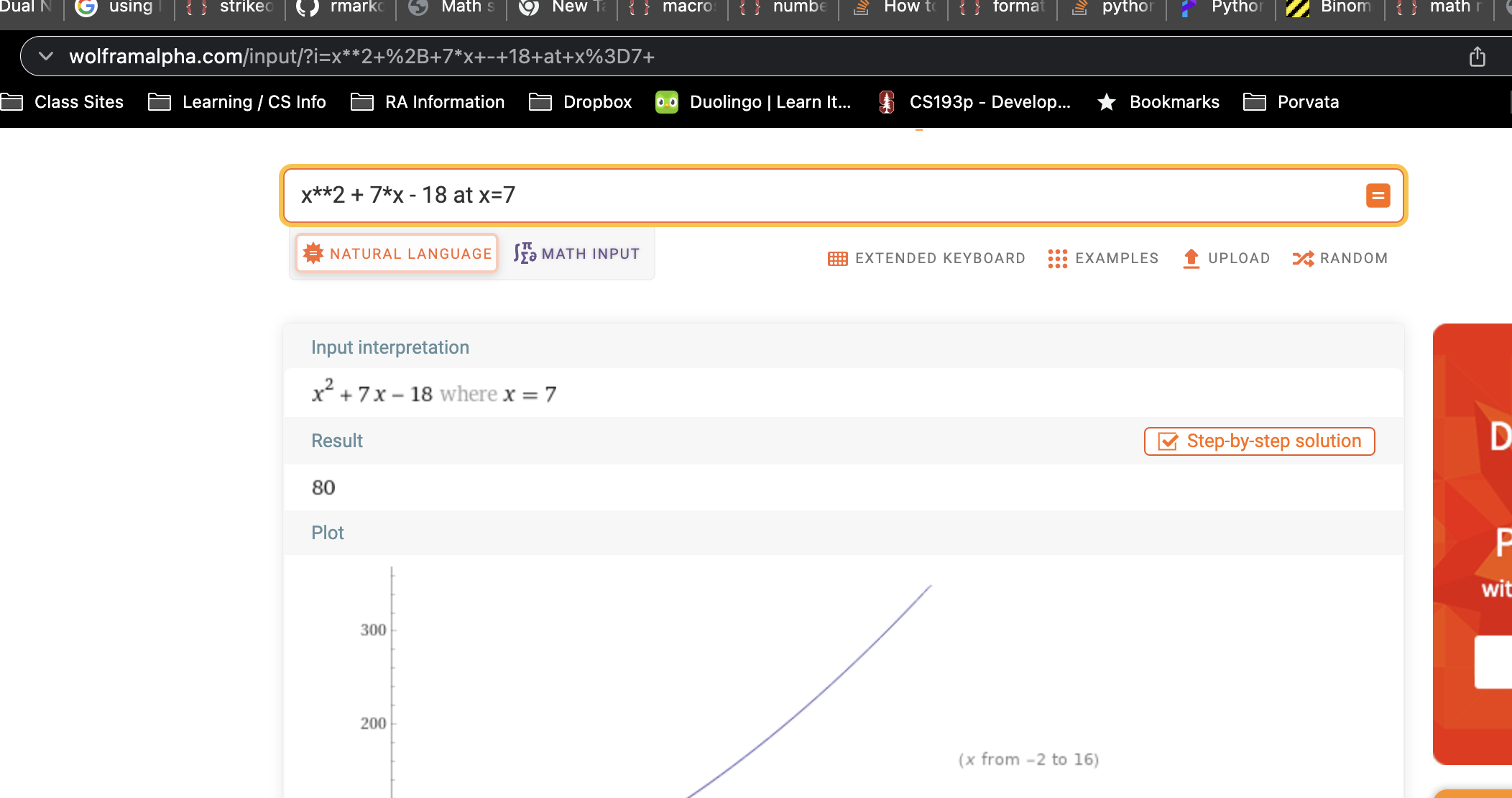
Let’s look at \(f(x) = x^2 + 7x - 18\) and evaluate the function at \(f(7)\). Totally made up function.

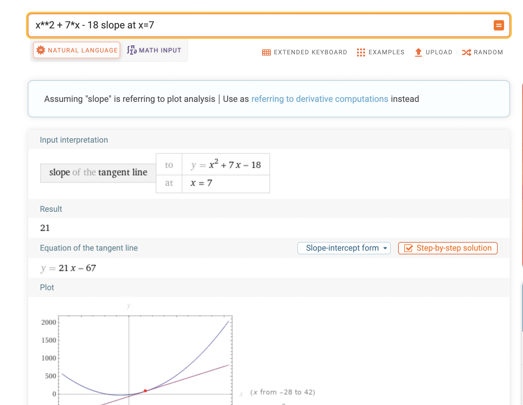
\(\begin{align*} f(x) &= x^2 + 7x - 18 \\ f(7) &= 7^2 + 7\cdot7 - 18 && \text{conver to dual first!} \\ f(7 + \varepsilon) &= (7 + \varepsilon)^2 + 7\cdot(7 + \varepsilon) - 18 && \text{reminder, we're basically adding 0 so it's fine!} \\ &= 49 + 14 \varepsilon + \varepsilon^2 + 49 + 7\varepsilon - 18 \\ &= 80 + 21 \varepsilon \\ \end{align*}\).

Beautiful! Instantaneous value and derivative (in this case slope). And grab a calculator or go to Wolfram Alpha. You can also get the value here and slope here. Also to prove I’m not lying!

value slope

Code

But obviosuly, why are we here?! The code!! So check out this whole example and a relatively nice (don’t love using eval (if you use it be cautious about performance! I just did it to get the printing functionality of the functions definition without using inspect)).

The code is linked here, but I’m also going to put the whole thing here because it’s not too long.

"""Class to demonstrate the power of duals"""


class Dual:
    """Class to implement Duals. For more information, see https://en.wikipedia.org/wiki/Dual_number"""

    def __init__(self, real_part, dual_part):
        self.real_part = real_part
        self.dual_part = dual_part

    def __add__(self, other):
        if isinstance(other, Dual):
            return Dual(
                self.real_part + other.real_part, self.dual_part + other.dual_part
            )
        if isinstance(other, (int, float)):
            # Just assume that they only want the real_part
            return Dual(self.real_part + other, self.dual_part)
        return NotImplementedError(
            f"{type(other).__name__} type not defined for addition with duals"
        )

    __radd__ = __add__

    def __sub__(self, other):
        if isinstance(other, Dual):
            return Dual(
                self.real_part - other.real_part, self.dual_part - other.dual_part
            )
        if isinstance(other, (int, float)):
            return Dual(self.real_part - other, self.dual_part)
        return NotImplementedError(
            f"{type(other).__name__} type not defined for subtraction with duals"
        )

    __rsub__ = __sub__

    def __mul__(self, other):
        # Check if it's a dual, otherwise handle it like normal scalar operation
        # If it's not a number, raise.
        if isinstance(other, Dual):
            # Foil baby
            # (a + b\eps) * (c + d\eps) = (a*c) + (c*b\eps) + (a*d\eps) + (b*d)(\eps)**2
            # But oh snap! Apply \eps**2 == 0
            # (a*c) + (c*b\eps) + (a*d\eps)
            return Dual(
                self.real_part * other.real_part, self.dual_part + other.dual_part
            )
        if isinstance(other, (int, float)):
            return Dual(self.real_part * other, self.dual_part * other)
        return NotImplementedError(
            f"{type(other).__name__} type not defined for multiplciation with duals"
        )

    __rmul__ = __mul__

    def __truediv__(self, other):
        if isinstance(other, Dual):
            dual_numerator = (
                self.dual_part * other.real_part - other.dual_part * self.real_part
            )
            dual_denominator = other.real_part ** 2
            return Dual(
                self.real_part / other.real_part, dual_numerator / dual_denominator
            )
        if isinstance(other, (int, float)):
            return Dual(self.real_part / other, self.dual_part)
        return NotImplementedError(
            f"{type(other).__name__} type not defined for division with duals"
        )

    def __rdiv__(self, other):
        if isinstance(other, Dual):
            return other.__truediv__(self)
        if isinstance(other, (int, float)):
            return Dual(other / self.real_part, 1 / self.dual_part)
        return NotImplementedError(
            f"{type(other).__name__} type not defined for division with duals"
        )

    def __pow__(self, other):
        # Just take into account the binomail expansion
        # but the beauty is we only need to worry about the first two terms.
        # Only works for numbers... don't wanna think about raising a dual to a dual
        if isinstance(other, (int, float)):
            return Dual(
                self.real_part ** other,
                other * self.dual_part * (self.real_part ** (other - 1)),
            )
        return NotImplementedError(
            f"{type(other).__name__} not defined for power with duals. Only int/float"
        )

    def __str__(self) -> str:
        return f"({self.real_part}, {self.dual_part}\u03B5)"

    def __repr__(self) -> str:
        return self.__str__()


def value_and_derivative_at_point(function_to_eval, point):
    """Wrapper around function to invoke and print helpful dual results"""
    result = function_to_eval.function(Dual(point, 1))
    value, deriv = result.real_part, result.dual_part
    print(f"For function {function_to_eval}, f({point})={value}, f'({point})={deriv}")
    return value, deriv


class GeneralFunction:
    """Abusing eval so we can see our function definition"""
    def __init__(self, definition):
        self.definition = definition

    def __str__(self):
        return self.definition

    def function(self, x):
        """Evaluate our expression. Note, x (arg1) is used in the expression."""
        return eval(self.definition)


if __name__ == "__main__":
    x = Dual(4, 3)
    y = Dual(5, 7)
    print(f"x: {x}")
    print(f"y: {y}")
    print(f"x + y : {x + y}")
    print(f"y + x : {y + x}")
    print(f"x * y : {x * y}")
    print(f"y * x : {y * x}")
    print(f"x - y : {x - y}")
    print(f"y - x : {y - x}")
    print(f"x / y : {x / y}")
    print(f"y / x : {y / x}")

    func = GeneralFunction("x**2 + 7*x - 18")
    value_and_derivative_at_point(func, 7)

Useful Resources

Here are a couple of other useful links I used to read up on Duals

Notes:

I couldn’t find a clean way to include a Latex package in Markdown so I was forced to use coloring to denote cancelling, but a better route would be to use the ulem latex package.

Dual Numbers and Automatic Differentiation

Background

Code

Mathematical Introduction

Benefits

Operations

Addition

Multiplication

Subtraction

Division

Exponents

Derivatives

Pitfalls

Real World Example

Code

Useful Resources

Notes: